

Introduction
Now I have a base understanding of both the properties of fluids and the ocean toolset within Houdini I will move on to the third and final tutorial I will be using for this section of my research – Houdini: Intermediate Ocean FX (Pluralsight, 2017) taught by FX Supervisor Andreas Giesen. Building on the previous course, this tutorial set teaches you how to set up a dynamic ocean from scratch without using the shelf and how to set up an object floating in an ocean which can then be turned into a full scene.
Creating a large scale ocean
Houdini 16 has a number of new options for creating ocean simulations compared with previous iterations of the program meaning that this lesson will be my primary source of reference as the previous two both use Houdini 15. Giesen runs through the “Small” and “Large” Ocean shelf tools to demonstrate the node networks that get automatically created when using the shelf defaults before demonstrating how to make an ocean network from scratch.
What constitutes an Ocean?
In Houdini, an ocean is made up of a series of key nodes:
- Render Grid: This determines the eventual size of the ocean and will be rendered at the end, make sure this node always has the render flag on it by ctrl+left clicking .
- Preview Grid: A way of visualising a small scale version of the final ocean but with a much shorter sim time, give the rows and columns the parameter: 2^ch(“../ocean_spectrum1/res”) in order to optimise the simulation . This node is plugged into the left input of the Ocean Evaluate node.
- Ocean Spectrum: This is where the majority of parameters effecting the ocean are controlled, here you can define the resolution, the size of the repeating pattern, as well as control the wave size, speed (number of big waves) and direction through the Wind and Amplitude tabs. Through the Mask tab you can break up the repetitive patterns by adding noise and a new feature of this node is the Wave Instancing tab which I will over in more detail later. This node is plugged into the right input of the Ocean Evaluate Node.
- Ocean Evaluate: Combines the Preview Grid and the Ocean Spectrum to create a coherent ocean by deforming the geometry of the grid using the settings dictated in the Ocean Spectrum.
Through these 4 key nodes a basic ocean scene can be created and manipulated at will, however there is considerably more to add to create a detailed and photoreal ocean scene as we will see.
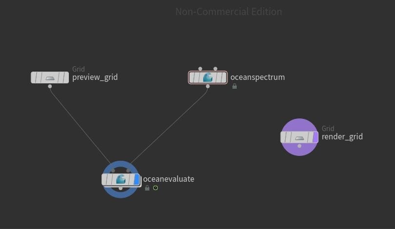
My node network after creating the four basic ocean nodes.
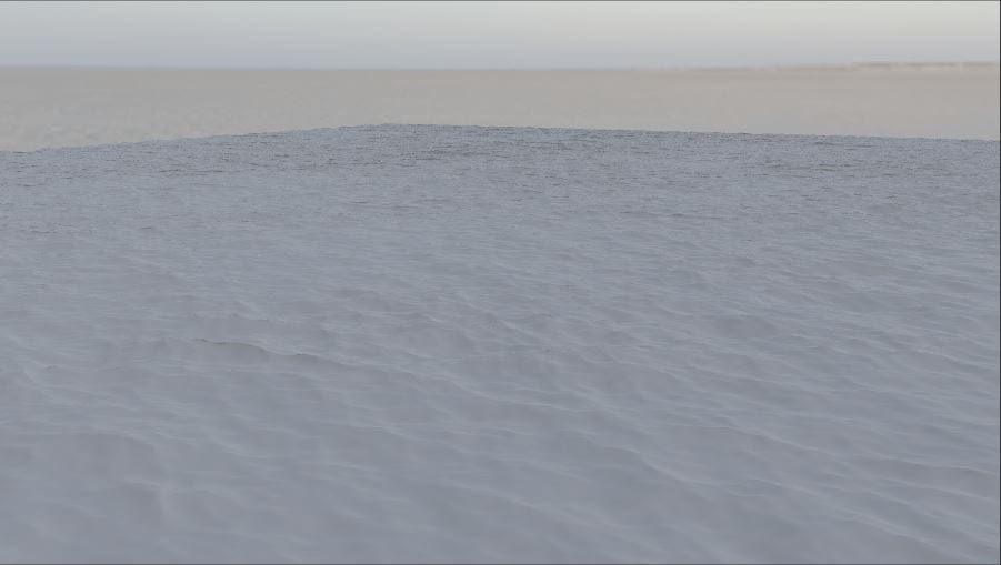
My initial ocean with the first Ocean Spectrum.
Layering Ocean Spectrums
Oceans in the real world are not uniform in their appearance due to a number of environmental factors including ocean depth, wind patterns and floating objects, this characteristic can be replicated by layering ocean spectrums in the ocean_surface network. By creating a second Ocean Spectrum node and connecting it to the same input as the original spectrum by way of a Merge node a second set of commands for waves can be added to the ocean – in the tutorial Giesen uses this feature a number of times, firstly to create the “low frequency” (large, infrequent) waves.
By greatly increasing the grid size of the second spectrum it will stop the new set of waves repeating as much as the base to avoid an ocean full of huge waves. Then, by enabling the “min wavelength” option, any small waves can be filtered out leaving only the low frequency waves desired.
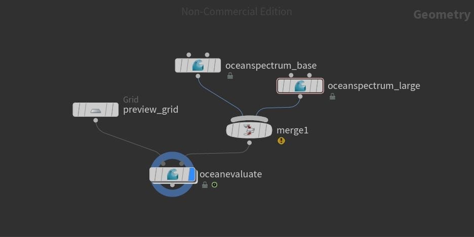
My network after layering in the second Ocean Spectrum.
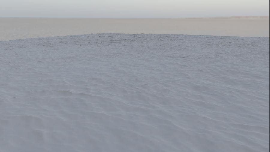
The second Ocean Spectrum adds a few large waves to the scene.
Wave Instancing
As I mentioned, a new feature in Houdini 16 is the Wave Instancing tab of the Ocean Spectrum node, this node allows you to create patches of specific waves scattered across your ocean. In order to do this, first you must scatter points within the ocean for the waves to be attached to using a Scatter node, plugged into the output of your render grid, with the number of points scattered increasing with the size of the render grid; this should then be plugged into a new, third, Ocean Spectrum Node. The Ocean Spectrum node has two inputs, the “Wave Instancing Points” (left) and the “Mask” (right), as the Scatter node is defining where to map the instanced waves to it should be plugged into the left input. Merge the third spectrum in to add this third level of waves to the simulation.
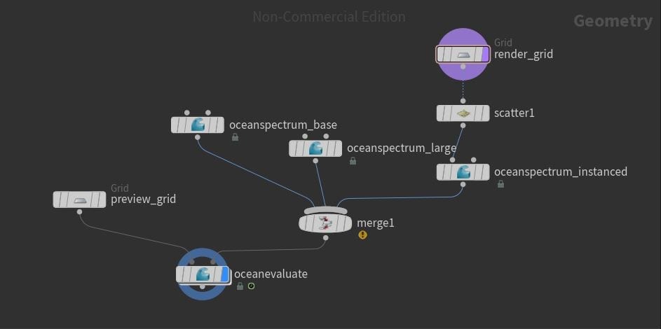
My network after adding the wave instancing Ocean Spectrum.
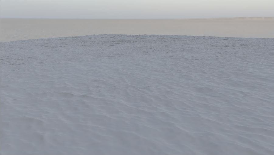
The wave instancing adds collections of extra waves scattered across the scene.
Faking Wave Interaction
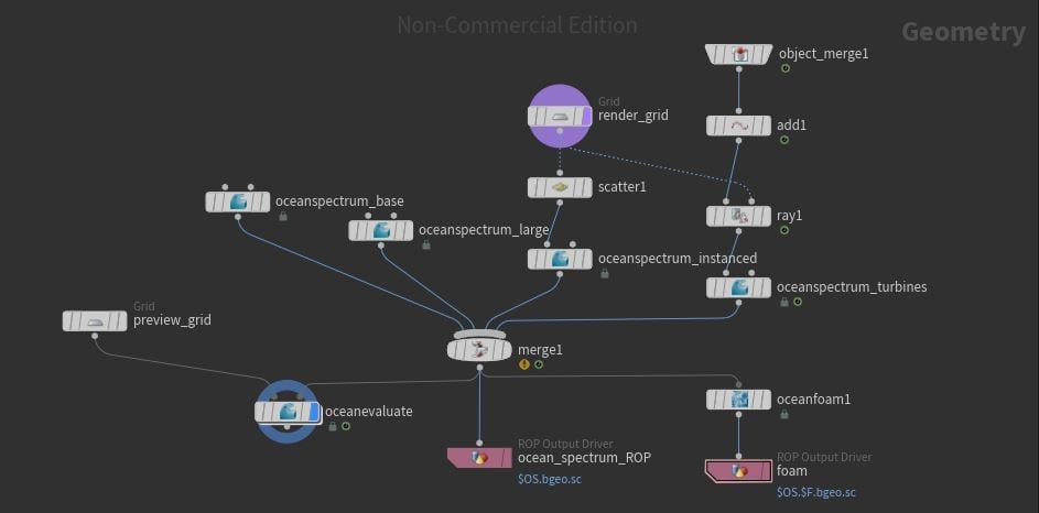
Giesen then adds a fourth Ocean Spectrum node to fake some interaction between the ocean and the turbine objects scattered across it. Firstly the points for the fake interaction to be mapped to need to be added to the network which can be done by using an Object Merge to bring the turbine geometry into the network and then an Add node to isolate a single point per turbine. In this case the points were far too high off the ocean surface and so, using a Ray node (with the turbine points plugged din on the left and the render grid on the right), Giesen moved them down to be level with the grid. This is then connected to the left input on the fourth Ocean Spectrum – which is subsequently added to the merge – adding waves to the base of each turbine.

The network after adding the 4th and final Ocean Spectrum.

This Ocean Spectrum adds small circles of waves around the bottoms of where the turbines will sit.
Rendering the practice ocean
In order to render out the final composition six things are required:
- Camera – this is really simple to add, simply frame the composition in the viewport and then use the drop down menu at the top right of the window to add a new camera. This will create a camera node which can be customised to fit the production specs.
- Light – essential to appropriately shade your composition. In this case Giesen uses an environment light to give the shot a base level of illumination, as well as a distant light that works similar to a very wide angle spot light to simulate the sun. Both of these can be added from the shelf and create their individual fully customisable node.
- Ocean Volume – This network is comprised of an Object Merge to merge in the Render Grid from the ocean_surface and an extrude volume to then give the render grid some depth (10 metres in this case).
- Shaders – In the materials tab, find the Ocean Surface and Volume material builders and drag and drop them in (any other geometry that needs texturing should also have materials isolated here). To apply these materials click on the ocean_surface and ocean_volume geometry networks and under the Render>Materials tab find the corresponding material and assign it. If particularly big waves are being used in the simulation it is important that the Min/Max Wave Height in the Ocean Surface Material has been increased accordingly. It is also important to toggle “Add bump to ray-traced displacements” on and adjust the Displacement Bound if it is not enough for your render (this can be determined by experimenting with test renders and adjusting accordingly).
- Writing out spectrum data – As the ocean_spectrum is using displacement to generate the waves, this must be written out using a “ROP”, this can be done by attaching a ROP_Geometry node to the output of the merge node in the spectrum network. Always change the output location so that the middle section reads “$HIPNAME/$OS/$OS.” as this will keep your cached .bgeo files in their own separate folders. Click save to disk to output the cache then in the Ocean Surface Material>Displacement>Spectrum Geometry tab browse and assign your spectrum data you just cached, as well as in the same location in the Ocean Volume Material.
- Mantra – Mantra is the rendering engine used by Houdini and is required to render out any simulations to video. In the Out context place down a Mantra node choose the appropriate camera and set the Engine to PBR (Physically Based Rendering) and adjust the Sampling/Shading parameters accordingly.
Then you are ready to render out your composition, simply choose the mantra node if using the render view, or click render to disk in the node itself for the entire sequence.
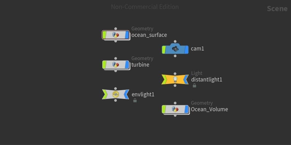
My 3 geometry networks, 2 lights and the camera.
The un-rendered visualisation of my scene so far.
Adding Foam to the ocean
At this point you could render out your ocean sequence as is however, in real life, waves on the ocean carry foam at their crest depending on the choppiness of the waves. To an extend this can be controlled by the Chop parameter in Ocean Spectrum node but, to create realistic foam, a Foam SOP, should be used, plug this into the output of your merge node.
Within the Foam SOP you first have to set the Region Type to Camera, and then increase the Z Far parameter in order to define the region you wish to add foam to. Other important parameters within the SOP include the Min Cusp which defines the minimum cusp value a wave requires to generate foam, the Min Velocity and Min Height do the same with their own respective values. Within the Solver tab Preserve Foam can be toggled, the effect of which will increase the life of foam in areas with a high foam concentration, essentially creating the realistic clumps of foam you see in real life. The last important parameter is the Particle Density of the Ocean Foam, this is controls the resolution the foam, the higher the value the greater the detail and render time. Finally create another ROP Geometry, attach it to the output of the Foam SOP and follow the previous process to cache out the foam to a .bgeo file.
As the final output for my portfolio will be a ship on a stormy ocean it is important to make the ocean look rough. Firstly this can be done by tweaking the base Ocean Spectrum by increasing the chop to give the waves bigger peaks, increasing the scale to make the waves themselves bigger and increasing the Directional Bias to align the waves with the wind more. Remember if you make a change to any node higher in the change than the ROP Geometry node you must re-bake (save to disk) the .bgeo file and update the link in the Ocean Surface Material to update your displacement.
Now you can go back into your Ocean Surface Material to the foam tab and assign the baked foam.bgeo file to the Foam Particles parameter. It is worth rendering it once and then tweaking the material settings to fit your desired style; parameters worth looking at are the Streak/Whitecap Intensity and the Foam Sharpness.
Once you are happy with the look of your foam you are ready to render out your final sequence, it is important to make sure you’re rendering the full frame range, not just the current frame and then you just have to click render to disk.
My final network of nodes in the ocean_spectrum network.
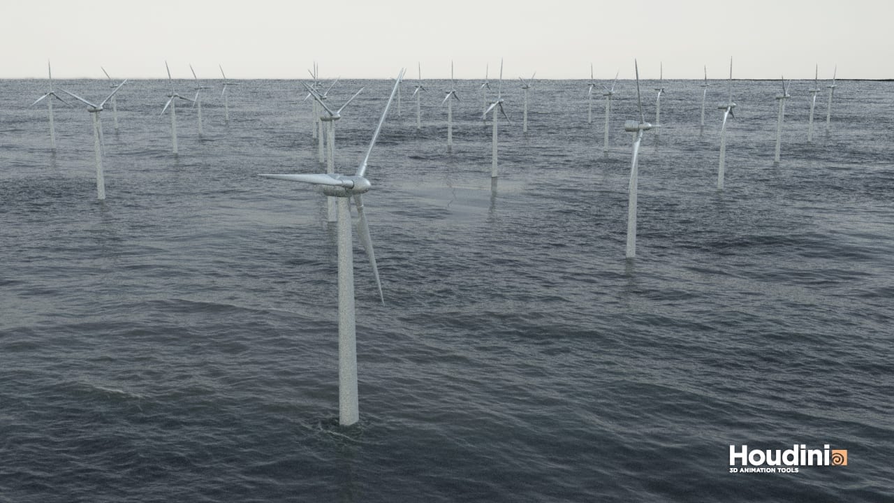
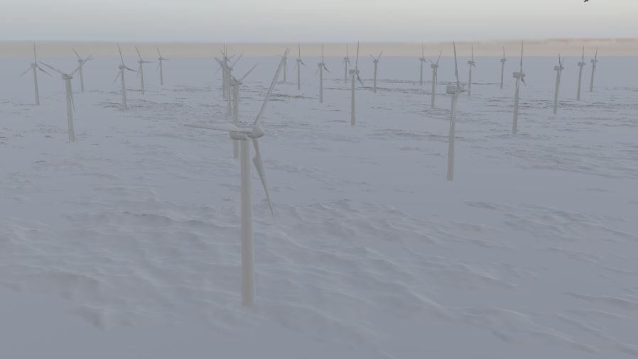
A rendered frame of my simulation created watching this tutorial.
End of part 3
That is the end of the first two modules of the Houdini: Intermediate Ocean FX tutorial, from this point Giesen goes on to discuss the simulation of a boat sailing on a rough ocean, which I will cover in the next post. For my I feel that I have a really strong idea of how oceans are created in Houdini and feel very familiar with the Ocean Spectrum node and how to stylise a realistic ocean.
References
- Pluralsight (2017) Houdini: Intermediate Ocean FX. Available from: https://app.pluralsight.com/library/courses/houdini-intermediate-ocean-fx/ [accessed 22 October 2018].