Learning To Create An Ocean – Simulating a Boat on an Ocean

Introduction

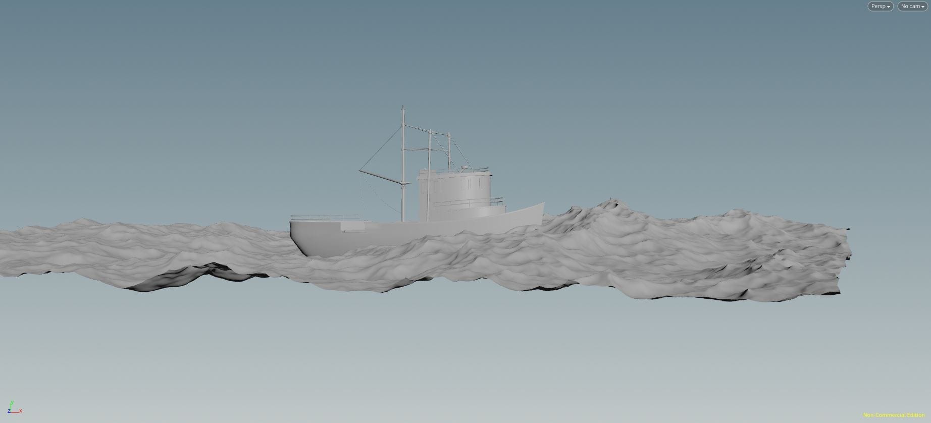
I am now on the fourth (and hopefully final) stage of learning how to simulate a boat on an ocean in Houdini 16 and in the second half of the Houdini: Intermediate Ocean FX tutorial I began in the previous post. By the end of this post I should be able to create a vast, realistic, ocean with whitewater and waves appropriate to the setting in which a boat can float and be affected by the waves and any other environmental factors I choose to add.

Starting with a boat

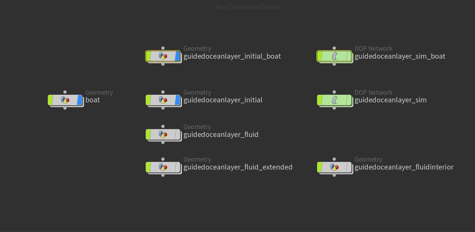
Giesen’s workflow in this tutorial is centred around beginning with the boat object, then building your ocean simulation from there so the first step is to set up a Geometry network for the boat and import the object’s file into it using a File node, from here use a new feature in Houdini 16 – the Guided Ocean Layer. By selecting the Boat_Geometry network and then the Guided Ocean Layer shelf tool all the nodes and networks required to start are created for you. Most of these nodes we have already covered in previous posts (Ocean Spectrums, Grids, Merges) so for more detailed information on those see my previous post. However the networks created by this shelf tool are the guidedoceanlayer_sim (AutoDopNetwork) that contains the solver and then four geometry networks: guidedocaenlayer_initial, guidedoceanlayer_fluid, guidedoceanlayer_fluidinterior and guidedoceanlayer_fluid_extended.

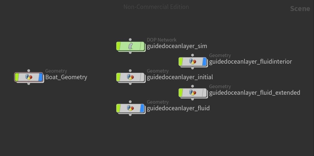
The object layer after using the Guided Ocean Layer shelf tool.

Guidedoceanlayer_initial

In this network is the very familiar Preview Grid, Ocean Spectrum and Ocean Evaluate that we created from scratch in the previous post however now this is connected to an Ocean Source node called the “Wave Tank”. The purpose of this is to limit what is generated to only what is required, to conserve memory. From this node is output particles (left output) and volumes (right output), the volumes connect to a File Cache – which I will cover further when we use them later – which then are split up into their specific type of volume, each leading to an output Null.

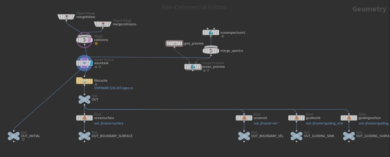
The guidedoceanlayer_initial network.

Guidedoceanlayer_SIM

In the AutoDopNetwork we have the place where the actual simulation happens. On the left is our boat geometry imported in and turned into an object through the use of a Static Object and Static Solver Node. On the right we have the FLIP Object node called the Guided Ocean Layer and the Gas Guiding Ocean Volume nodes, these essentially import all the particle and volume data from the GOL_Initial and, when plugged into the FLIP Solver, match the FLIP tank we create to house and manipulate the boat perfectly with the rest of the ocean as, remember, oceans in Houdini are created with displacement not particles.

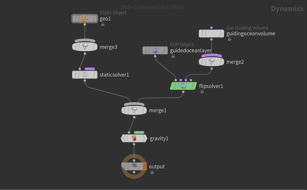
The guidedoceanlayer_sim network.

Guidedoceanlayer_fluid

All three GOL_fluid networks work by processing the simulated data form the GOL_sim. In this network, firstly, the DOP Import node brings in the simulation data from the AutoDopNetwork, this is then fed into a series of nodes that isolate the important data and compress it to maximise disk space before feeding into another File Cache. From here the network splits into, on one side you can preview the fluid surface in its current state using the surface_preview but this is only an approximation of the final output. On the other side you have a Particle Fluid Surface node that leads into another Cache and a render Null however these are not required unless you do not plan to use the wave tank within a wider ocean.

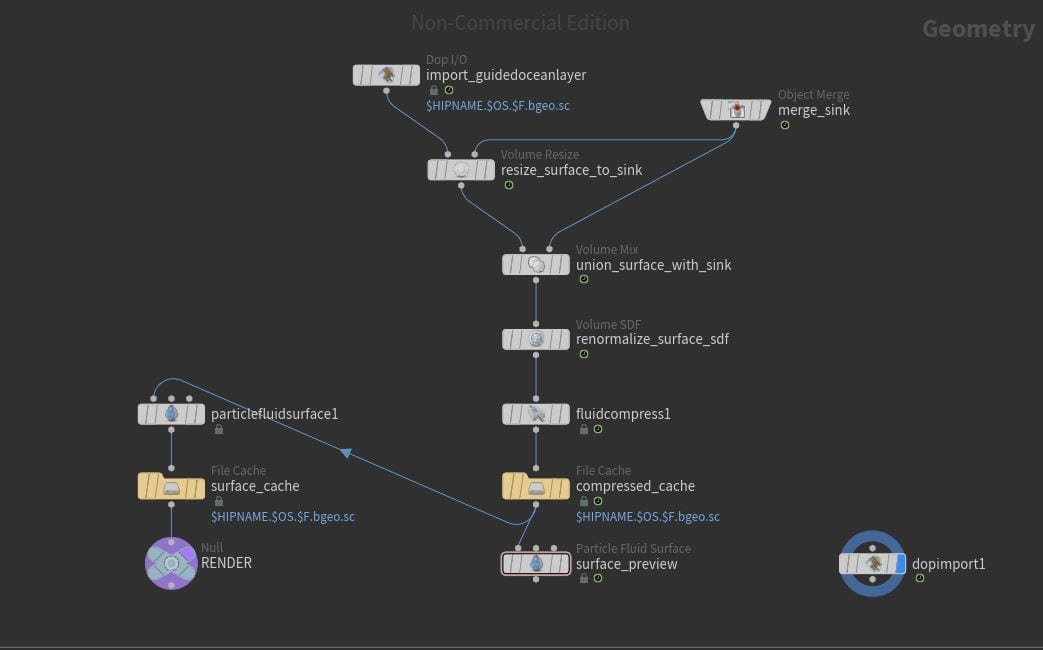
The guidedoceanlayer_fluid network.

Guidedoceanlayer_FLUID_ extended

It is this layer that will be rendered when we come to render out our final simulation at the end. This network is very similar to the previous one but with some additions, rather than just the Wave Tank the GOL_fluid_extended covers the entire ocean (hence extended), it does this by creating a mask and spectra that seamlessly blends the tank and the displaced layer.

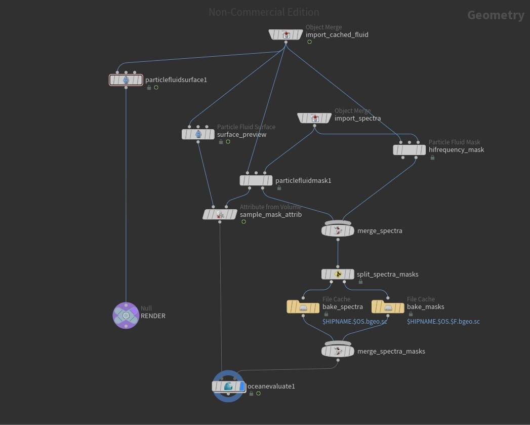
The guidedoceanlayer_fluid_extended network.

Guidedoceanlayer_FLUIDinterior

On this layer using an Object Merge node, the necessary data is imported so that later we can add the volume shader for rendering as we did in the previous post.

The guidedoceanlayer_fluidinterior network.

Waves in a storm

Now we have all of our nodes and networks the first step is to dive into the Ocean Spectrum node in the GOL_Initial network and edit the parameters to replicate stormy waves in our displacement. I covered in detail how to manipulate the Ocean Spectrum parameters in my previous post so will not rewrite all that here, however, during a storm the wind will increase and so it is important to up the directional bias to replicate this, and increase the chop to create the sharper tops to the waves that stop the simulation from looking too calm.

Custom waves

A new feature in Houdini 16 is the ability to add custom waves to shape the look of your ocean, do this by adding an Ocean Waves SOP node and connecting the output to the Merge node already connecting your Ocean Spectrum and Ocean Evaluate. One way of creating these custom waves is within the node, you will need to toggle the custom wave on by ticking the “number of waves” parameter and then there are a series of further parameters within the node to customise how the waves look, but for a little more control you can use a Grid and Scatter node and plug these into the left input of the Ocean Waves SOP.

Set up the Grid so that it is bigger than your preview grid with a few rows and columns and an offset centre to create a more randomised look. Below this the Scatter node will generate points on the grid, the default force count on the Scatter is 1000, this is far too many for our purposes as this will define the number of larger waves (Giesen uses 14). In order to make the waves move a Transform node is required, place this between the Scatter and the SOP and then, using key frames, have the points move from the front of the boat to the back in the same direction as your waves. Navigate to the Shape section of the Ocean Waves SOP and from here you can design the look of your custom waves. The Crest Width and Amplitude control the height, the Chop is the same as before, the radius affects the distance from your scattered points that is affected by the SOP.

Custom waves created just using the Ocean Waves SOP.

Custom waves created using the grid/scatter system. They are more subtle but far more realistic.

Simulating the boat motion

Preperation

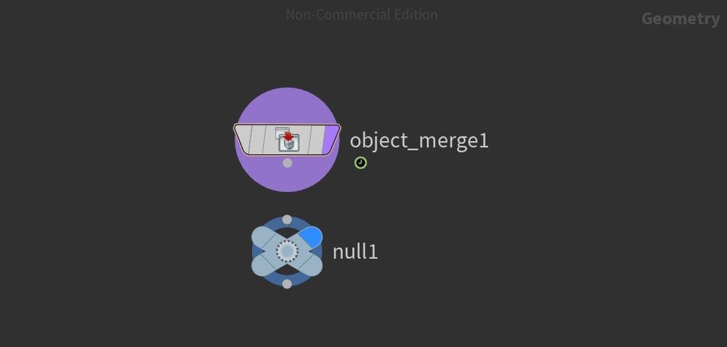
In order to make the boat react to the waves we have to first simulate it’s motion. This will be done in a separate simulation to the ocean so duplicate the GOL_Initial and the GOL_Sim this will duplicate all the nodes inside the networks and update their connections however in this case we do not want that for the Ocean Spectrum. This is because if we change any of the settings to our original Ocean Spectrum or custom waves we will also want these changes to be made in the duplicated boat simulations, or the motion of the boat will look unnatural. The solution to this is to use an Object Merge node to merge in the Merge Spectra node from the original GOL_Initial and replace the one in the new network; now any change made in one will apply to the other.

My object layer at this point.

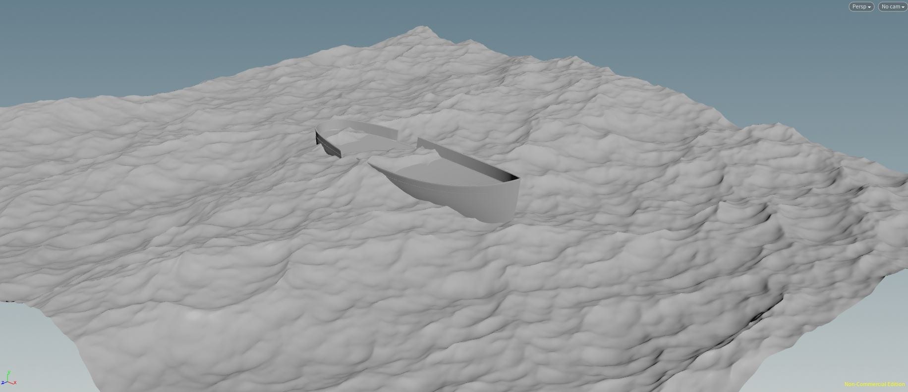
In order to simulate the motion of the boat on the ocean it needs to be turned from a static object into an active rigid body (RBD) object. However, not all the boat needs this as not all of it is submerged, instead we can isolate the main hull of the boat, simulate its motion, and then apply that to the entire geometry later. The first step in isolating this main body is attaching an Assemble node to the penultimate node in the Boat_Geometry network (whatever is currently above the render), and toggling on the Create Packed Geometry option. This will take every primitive that makes up the geometry of the boat and group them into coherent shapes; in Giesen’s tutorial he goes from 9000 primitives to 7 after using this process. Now, in the viewport, you can select the entire main body of the hull in one click, do this and press delete to create a Blast node that will remove the selection, then toggle on “delete non selected” to invert the process leaving you with just the main body. The last step before turning the boat into an RBD is deleting the static object (left) section of your GOL_sim_boat network as you don’t need it anymore, and making sure that you are simulating using the same network by clicking the dropdown menu in the bottom right of the Houdini interface.

To turn what’s left of the boat into an RBD make sure the Boat_Geometry network is selected then click the RBD Hero Object shelf tool. Now in your GOL_Sim_Boat network you will see the left side has been recreated but now with an RBD Object node at the top and a Rigid Body Solver at the bottom replacing the Static Object and Static Solver that you just deleted.

Before we solve the motion of the boat however it is important to check it’s collision geometry, this can be done in the RBD Object>Collisions>Bullet Data tab and toggling on the guide geometry which will display in blue. It is likely at first that the collision geometry will have only mapped around the outside of your boat and not taken into account any crevices or dips, this can be fixed by changing the Geometry Representation. It is worth cycling through the options to find whichever works best for your specific situation, however in this case “concave” is most appropriate.

The last thing to do in order to have your boat motion simulated is toggle on Feedback Scale (by changing its value to 1) in the Solver tab of the Flip Solver node otherwise there will be no interaction. Now if you play your timeline through, your boat will move on the ocean.

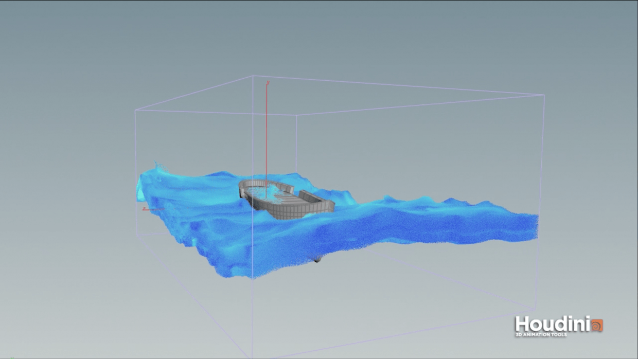
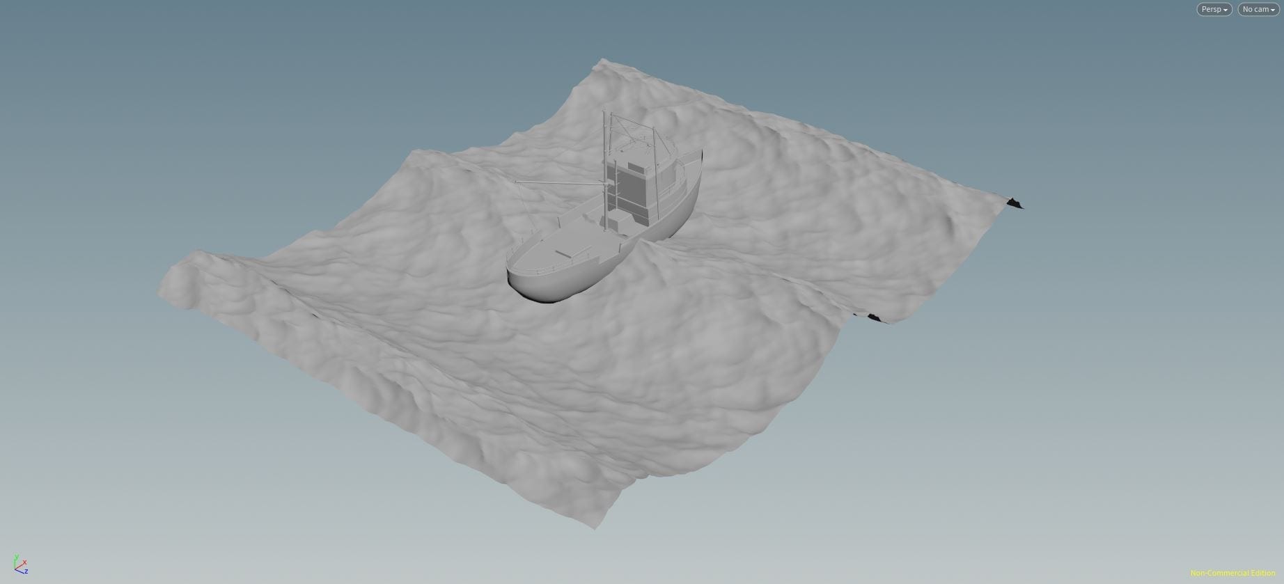
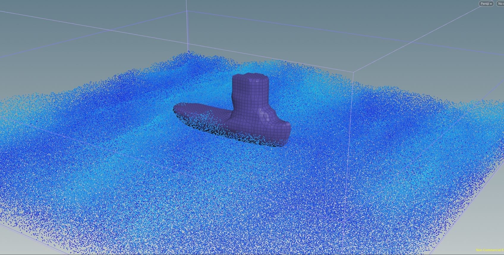
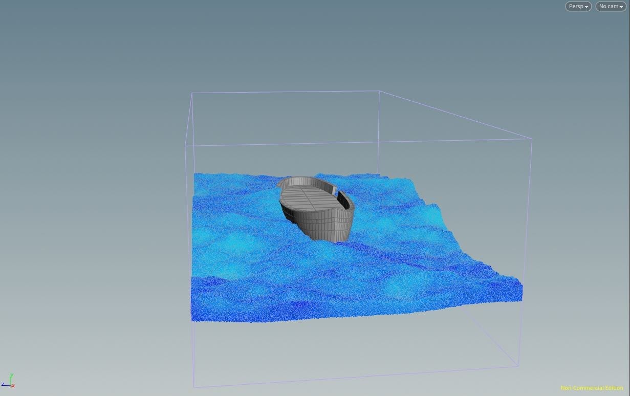
The isolated boat hull on the ocean.

Simulating

Or will it? As you will see, if you play your simulation out now the boat will affect the simulation particles however it will fall through the waves and leave a boat shaped hole in your ocean. To fix this we first need to look at some of the properties of our Wave Tank in the GOL_Initial_Boat network. Firstly, because this tank in this network is only effecting the boat, you can significantly reduce the size of the tank so that it surrounds the boat more tightly – we then need to animate the tank so that it moves, otherwise our boat will just sit motionless in the ocean. To do this, clear the current channels of the Centre parameter of the node, then move it forward in the x direction animating it with keyframes so that it will move during the simulation, it is also worth moving it down a few places in the y direction to leave room for depth. To add depth to your wave tank you have to increase the Layer Size, however this is linked via an expression to the Particle Separation which is, in turn, linked to the Particle Separation of the DOP network so you have to go into you GOL_Sim_Boat and decrease this value a bit – bear in mind this will increase the level of detail of your guided ocean layer and slow down your simulation times. Now the particle separation has changed you can go back to the Wave Tank and increase the multiplier for the Layer Size to give your ocean some depth. Giesen uses 20 for this, he also lowers the Guiding Surface Thickness, again to help with motion simulation.

Now your boat should be floating instead of sinking! The last couple of tweaks required here are in the Physical tab of the RBD Object in the sim. Firstly the centre of mass should be manually defined and move downwards slightly as well as increasing the density based on the size of your boat and lowering the rotational stiffness, otherwise the motion of your boat will look unnatural and the boat will not be properly effected by the waves.

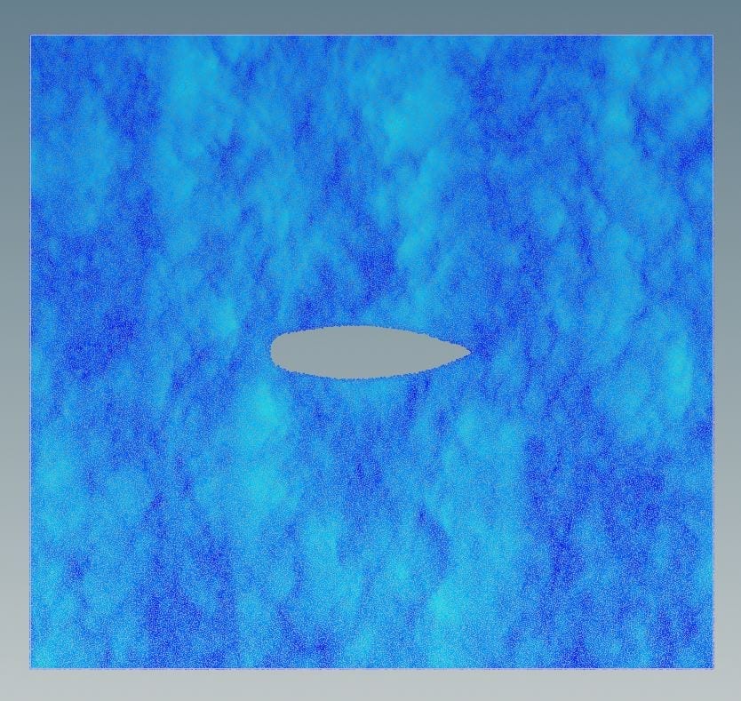
The boat sitting in the newly deepened Wave Tank.

Adding Velocity

In order to make our boat move forward on the ocean surface, we first need to add a VOP Force node to the GOL_Sim_Boat network between the Gravity and Output nodes. To make sure only the boat is being affected by the VOP and not the ocean set the Group parameter to “boat”. If we dive into the VOP node we can edit the VEX code and we are presented with in interface similar to the node workflow in Blender where all an object’s various properties can be manipulated via nodes.

To make the boat move we need to add a constant force in a direction so drop down a Constant node, change the type to Vector and add a positive value in the x direction (Giesen uses 500000). Connect this to the Force parameter of the VOP Force Output node and your boat will now move forwards however currently the constant is being continuously added meaning that by the end of the timeline your boat will be going much too fast. To fix this first drop down a two way switch; connect the Constant to Input 1, then duplicate your Constant but with an x value of 0 and make it input 2 before connecting the Result to the Force parameter of the output. Now we have the two values we need to set a condition, place a Vector To Float node and a Compare node down and add them to your network so it goes VOP Force Global (v)>Vector To Float (fval1)>(input 1) Compare>(condition)Two Way Switch. We can now set the condition that will stop adding force to our boat by changing the compare node test to Less Than Or Equal and setting the Compare To Float value to 2.6. The Vector To Float node converts the velocity of the object to an arbitrary value and so depending on the size of your boat this value may change however the effect of this now is that velocity will only be added if the float value is less than or equal to 2.6.

The interior of my VOP Network.

Caching

I have mentioned caching a couple of times already, now it is time to create our first cache. In order to minimise sim times, now we are done tweaking the boat’s motion, we can write out what the boat will be doing on every frame to the disk and then import this back in using a File node. A cache wasn’t automatically generated for us for our boat so jump into the Boat_Geometry network, duplicate the DOP Import node that has been created and change the Import Style to  “Create Points to Represent Objects” – this way we don’t have to write out the entire geometry, just a single point that we can then parent the boat geometry to. Connect this DOP Import to a ROP Output Driver, make sure it’s set to render a frame range not just the current one and then save it to your disk.

As I said, to import this file back in, create a File node in the same network and locate the cached .bgeo file. This will only import that single point though, to reconnect the geometry we will use a Transform Pieces node. On the first input we need to add our static boat geometry, so connect the output from the Transform node to the left input, and then add the point data from the File node by connecting it to the middle input. If you display the Transform Pieces now we will have our isolated boat motion and not have to worry about simulating it in any further tests. It is important to remember that if you change any of your base ocean, wave, or boat settings this motion will need to be re-written out and re-imported back in otherwise the boat will not adapt to the new ocean.

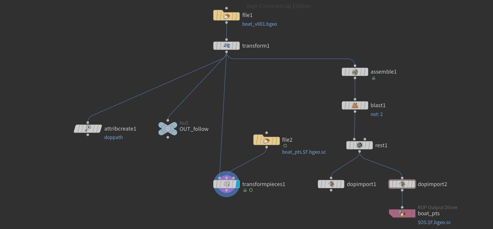
The interior of my Boat_Geometry network after baking the ROP and importing it back in.

Collisions

To create an accurate interaction between the boat and the ocean the boat needs to effect the water in our high-res ocean simulation (GOL_Sim), we will do this by optimising the collision geometry of the boat. Working now within the GOL_Sim not the Sim_Boat, firstly toggle on the Use Deforming Geometry option on the Static Object node or there will be no collision; one method is to decrease the Particle Separation of the guided ocean layer FLIP Object, as you can see if you toggle on the collision visualisation and jump to the second frame this will refine the collision geometry of the boat and make it more accurate.

The collision geometry before any modifications are made. It’s smooth and very inaccurate.

This, however, is a very slow process and is quite taxing on the memory so we will use option 2. Again we can delete the static object side (left) of our GOL_Sim as they will be replaced, then select your Boat_Geometry network and click the Deforming Object shelf tool. Dive inside this network and you’ll see a few nodes have been added below the Transform Pieces: a Collision Source, an Attribute Create, a File Cache and a Null. Similarly, in the GOL_Sim the left side has been recreated adding what looks like the nodes you just deleted, however these nodes have been set up differently meaning now we control the collision geometry from the boat network allowing for increased refining.

Now we have this new set up the first step is to toggle on the Collision Operation option in the FLIP Object node and link it to the Division Size of the Static Object by copying the parameter and pasting the relative reference; this way we don’t have to waste sim time by creating an unnecessarily high resolution collision geometry when we lower the Particle Separation.

Just like when isolating the boat’s motion, because the boat isn’t fully submerged, we only need to generate collision geometry for the hull of the boat so the first step to refining the collisions is to move the left input connection of the Transform Pieces back onto the output of the Rest node. If you place the display flag on the File Cache at the moment you will see the low res collision geometry and notice that at any thin areas the collision looks warped and unnatural as the VDB generation is struggling. Rather than just increasing the collision resolution we can instead just modify our collision object to make the thin areas a little thicker.

If you remember we turned our boat into packed geometry so we cannot select the individual primitives that make up the hull, to change this back now add a Convert node below your Transform Pieces node and now you can select your individual primitives again. In the viewport, select any faces that need to be make thicker then, with the mouse still in the viewport, drop down a Poly Extrude node (press TAB and search) which will create the corresponding node in your network with only the selected primitives assigned. Now change the Divide Into tab to Individual Elements and increase the Distance parameter until the are the required thickness. Now if you check your File Cache again the VDB should look much better.

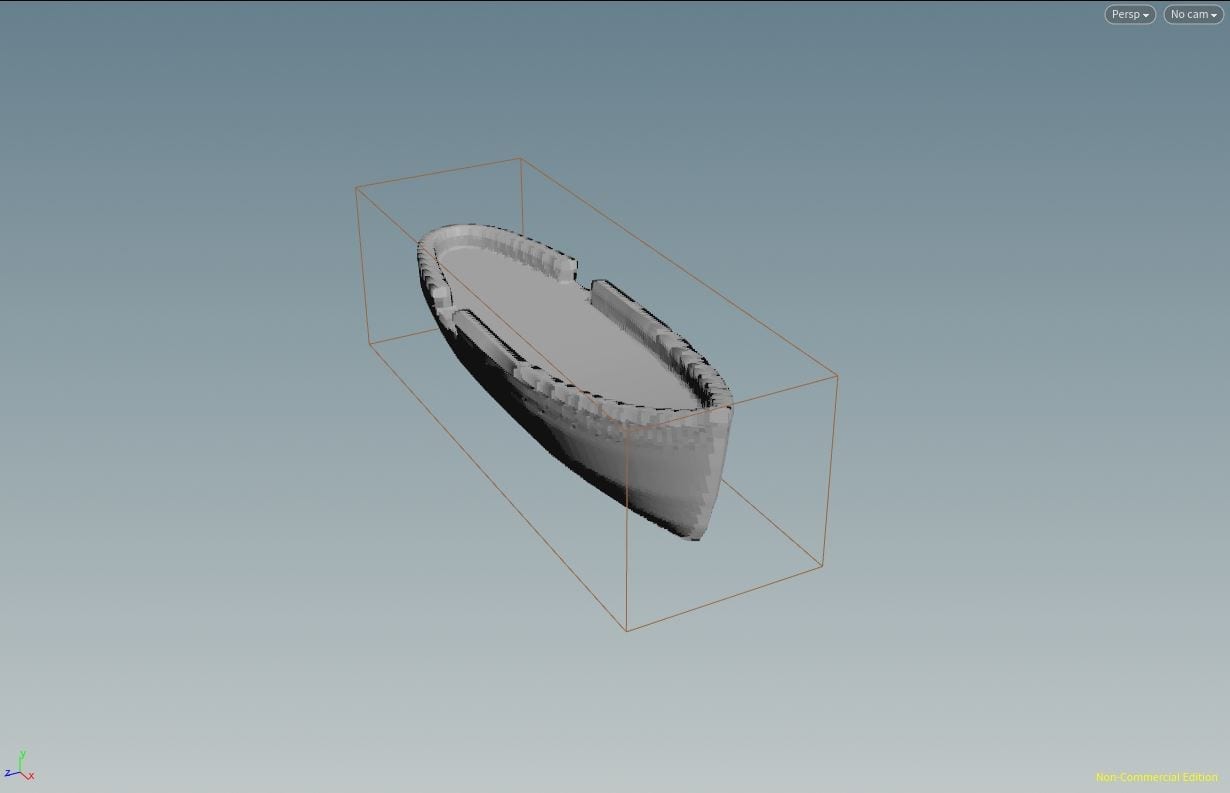
My collision VDB. Compared to the previous image this collision is very detailed.

In the tutorial however, because of the dips in the side of the boat, water is being created on top of the boat geometry which must be fixed. To do this first move the Attribute Create 1 and OUT_Follow nodes down so that they are connected to the output of the Convert node or we won’t be able to select their primitives. Then repeat the extrude process, selecting all the primitives on the top face, and create another Poly Extrude, this time placed between the Convert and the OUT_Follow Null. Remember this is just the collision geometry, not what the boat will actually look like, so you can extrude it up quite a bit and not have to worry about it looking odd. Now if you look in the GOL_Initial and view the Wave Tank you will see the particles no longer spawn above the boat. Lastly, while you’re in the Wave Tank, if you can afford to make the tank any smaller then do to maximise simulation speed and also, because the ocean is stormy and the boat will be moving a lot, you should significantly increase the layer size (Giesen changes the multiplier to 16) and then move the tank down to compensate.

At this point it is worth caching out your Wave Tank using the File Cache node below it to conserve simulation time in a similar way to how we cached out the boat motion. This time however we will just use the File Cache node. It works the same as the ROP Output Driver, just make sure it’s set to render the frame range not just a single frame, set up the path to your desired location and then hit render to disk. Like before, to import this back in, drop down a File node, locate your cache, and move all the connections below the File Cache (in this case just the Null) onto the new File Node.

My Boat_Geometry network after adding the collisions.

My GOL_Sim Network (without the boat displayed) now I have added accurate collisions.

Optimising the HIGH-RES FLIP SIMULATION

We’ve nearly finished creating our boat and ocean, there are only a few more steps left before we add the whitewater and prepare the scene for render.

Firstly, jump into the GOL_sim network and lower the particle separation even further until you’re working in hundredths, this will increase your sim times, but it is necessary for a detailed simulation.

Next, in the FLIP Solver navigate to the Particle Motion>Droplets tab and toggle it on. Droplets are particles that are separated from the main fluid, by toggling this feature on we can set the threshold for what is considered a droplet and what is not. Currently the parameter is set to “Blend With Fluid” which just means that the droplets will rejoin the main fluid when they collide back with the surface – this is what we want so leave this option for now.

Now we can look at the Volume Motion tab; most of these parameters are already set to what we want, however if we navigate to the Collisions section there are some options to manipulate. Change the Velocity Type from Point to Volume as, while we may get more detailed splashes from point, most of the detail for our splashes will be coming from the whitewater and so Volume is more appropriate here. Also increase your Velocity Scale if you want bigger splashes (which we do) and decease the surface extrapolation just to make sure that the particles do not stick to the curves of your boat collision. Then in the Solver tab if you have a multicore machine then disable Use Preconditioner to make use of all the cores.

My GOL_Sim network with the boat displayed.

You are now ready to Flipbook your simulation and check whether any of these parameters need further tweaking to get the best look for you. Before you simulate, in the FLIP Object>Creation tab disable Allow Caching otherwise the simulation will fill up your memory but remember to toggle it on again afterwards. One way to do this is create a second “sim” take with all your settings for simulation and rendering there so you can flip back and forth at will. To see what your ocean will look like as a mesh, not just the particles, in your flipbooks go into the GOL_fluid network and cache out the “Compressed_Cache” File Cache using the process we have already covered and import it back in with a File node, plugging the nodes under the Compressed Cache into the output of File node now instead.

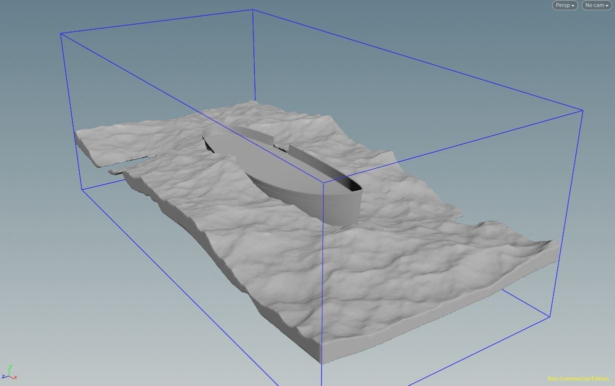
My GOL_Fluid network displaying the fluid meshed over my simulation. This is as accurate a representation of the waves we can get pre render.

End of part 4

I said at the beginning of this blog post that this would hopefully be the last section of the Learning To Create An Ocean set of posts, 4034 words later we still have to create the whitewater and prepare the scene for render which I will do each in it’s separate part 5 and 6 post. The simple fact is there are a lot of steps to creating a realistic ocean simulation and as Houdini is such a complex program I would not be doing the process justice if I simply provided a step by step list of what to do without explaining the purpose and function of each of the steps first.

REFERENCES

- Pluralsight (2017) Houdini: Intermediate Ocean FX. Available from: https://app.pluralsight.com/library/courses/houdini-intermediate-ocean-fx/ [accessed 24 October 2018].