
Introduction
At stage 5 we now know the basic principles of fluids in Houdini, how the oceans work using displacement and how to combine them together as well as simulating an object floating and moving in them. In the last post we set up our ocean, the tank for our boat, created the actual motion for a boat, fixed it’s collision geometry and then tweaked our simulation. At this point we could render out our simulation and it would look like a coherent scene however it would not look photoreal. As we have already seen, in stormy weather, oceans have a lot more whitewater and, when objects move through water, foam spray and bubbles are created. We will now set this up for our simulation.
The Whitewater Shelf Tool
You can create the whitewater from scratch as we have done previously using the Foam SOP but because of the amount of networks we have already, the number of connections we would have to set up would be large and (thanks to the shelf) unnecessary. In the Oceans tab of the shelf click the Whitewater button then navigate into your GOL_Sim and click on the FLIP Object node entitled “Guided Ocean Layer” and with the mouse in the viewport press the Enter key and a number of new nodes and networks will be set up.
Two of these networks we have seen before in part 2 of this series: the whitewater_sim and whitewater_source however this time, instead of the whitewater_interior there is the whitewater_import.
whitewater_import
While it bears a different name to the whitewater_interior we used in part 2, the function of the import network is exactly the same. First it imports in the data from our simulation, then rasterises it so we can apply a material for rendering.
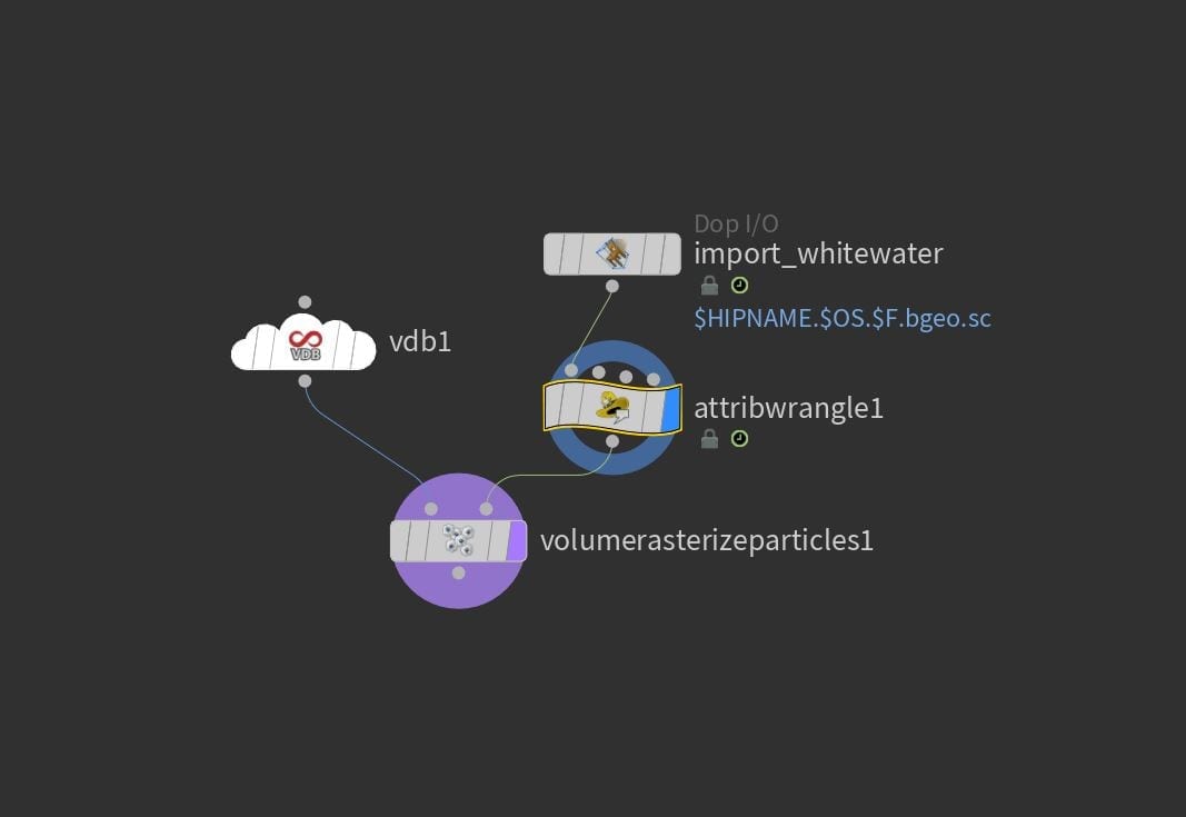
The whitewater_import network.
Whitewater_source
This is where the points for our whitewater are generated to be sent to the simulation. As we have cached our compressed GOL_Fluid we need to relink the Object Merge to the File node that imported our cache back in to the network. Below the Whitewater Source node is another File Cache as it is recommended to cache out the whitewater source before simulating it to cut down on sim time.
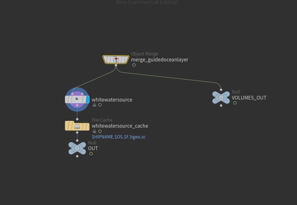
The whitewater_source network.
Whitewater_Simulation
Here we have a pretty standard simulation AutoDopNetwork, a Whitewater Object and a Whitewater Emitter that import in the data from the whitewater_source and then connect to the Whitewater Solver where most of our adjustments will be made, before connecting to a Merge and an Output. There is quite a lot we need to add to this network to make it up to date with our other simulations – primarily the collisions with our boat that we set up in the previous post.
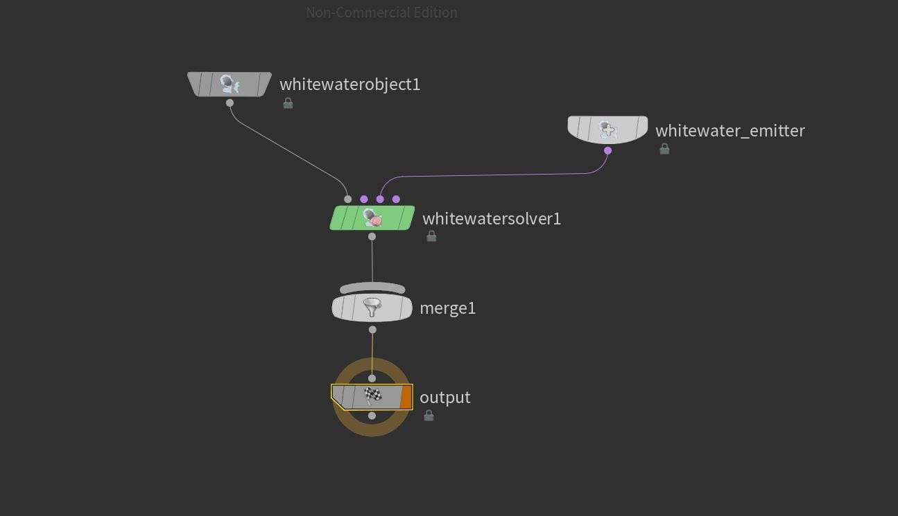
The whitewater_sim network.
Tweaking the networks
Whitewater_Source
The whitewater source node is the first thing we need to define in order to create a realistic whitewater simulation, skip forward a few frames to see what we are working with. The way in which the whitewater points are created is decided through ramps, with a minimum and maximum value for Emission, Curvature, Acceleration and Vorticity and whitewater being generated based on a range of values corresponding to these attributes.
Emission – Currently the Min and Max values of the emission are already fine, however as we cannot see below the surface of our ocean we can toggle on the Limit By Depth option meaning that emission points will only be generated above the surface, but increase the Max Depth just a little to compensate for this.
Curvature – The curvature is currently emitting very few points (as you will see if you temporarily disable the other emitters) so lower the Min Curvature a bit. Other than this, all these parameters are fine how they are.
Acceleration – This generates most of the emission points as our boat is moving relatively quickly. Again just lower the minimum value, this is a stormy ocean remember, so there should be a lot of whitewater and this will mean the low frequency waves will also carry foam.
Vorticity – In simple terms, vorticity measures spinning. We do not have much spinning in our ocean scene as there are no whirlpools or drains so this tab isn’t especially important. Nevertheless, there will be some vorticity in our scene so again lower the Min Vorticity slightly.
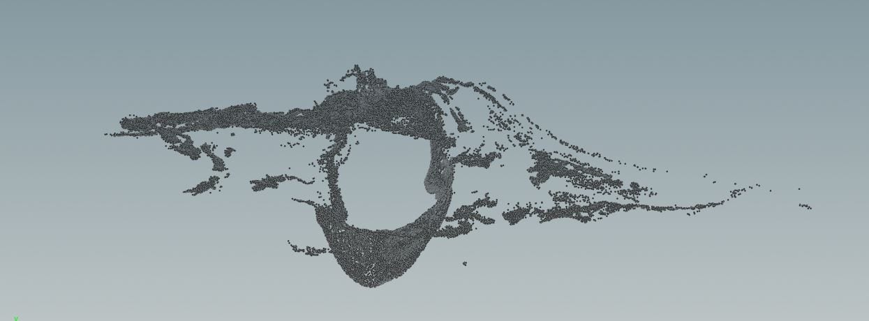
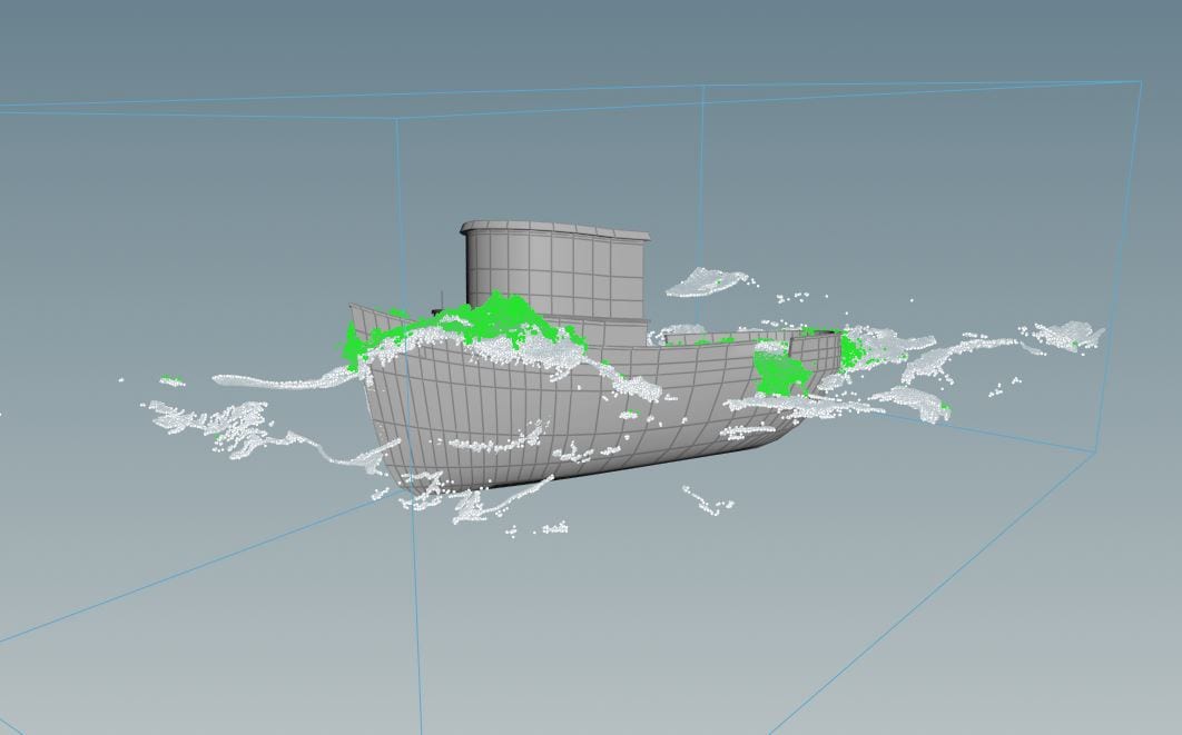
A screenshot of the viewport before we add a POPVOP.
As we created out whitewater from the shelf all the corresponding paths have already been set up so, for now, we are done with the Whitewater Source node. However, Giesen makes the point that at the moment the whitewater generation looks quite uniform and unrealistic and so explains how to add some noise to the emitter generation to remedy this. Only one node needs to be added to the whitewater_source to add a little more randomness to our emitter generation: a Point VOP node after the Whitewater Source.
Within the Point VOP
We have already dealt with VOPs once before in order to give our boat some motion so the interface should already feel familiar. To add noise jump into the VOP and connect a Turbulent Noise Node to the input via the Position (P) parameters. Change the type of noise to Original Perlin Noise, increase the Roughness and Frequency in the x axis while decreasing the Frequency in the y and z axis as we don’t want any decreased particles above or below the surface.
As we are trying to add noise by deleting some of our existing points rather than by adding them we also need to set up another Two Way Switch so create one and a Compare node set to Less Than Or Equal To and lastly a Remove Point node. Connect these to your VOP network so the connections run Turbulent Noise > (input 1) Compare > (condition) Two Way Switch > (ptnum) Remove Point and Geometry VOP Global (ptnum) > (input 1). As you can see if you switch the Point Remove on and off this is now breaking up the uniformity of the Whitewater Source. To further randomise this noise, right-click the Offset parameter of your Turbulent Noise and promote the parameter then, if you add the expression “$F/10” to the Offset parameter of your VOP Noise it will move the noise over the course of the simulation adding another random element to break up the Whitewater Source.
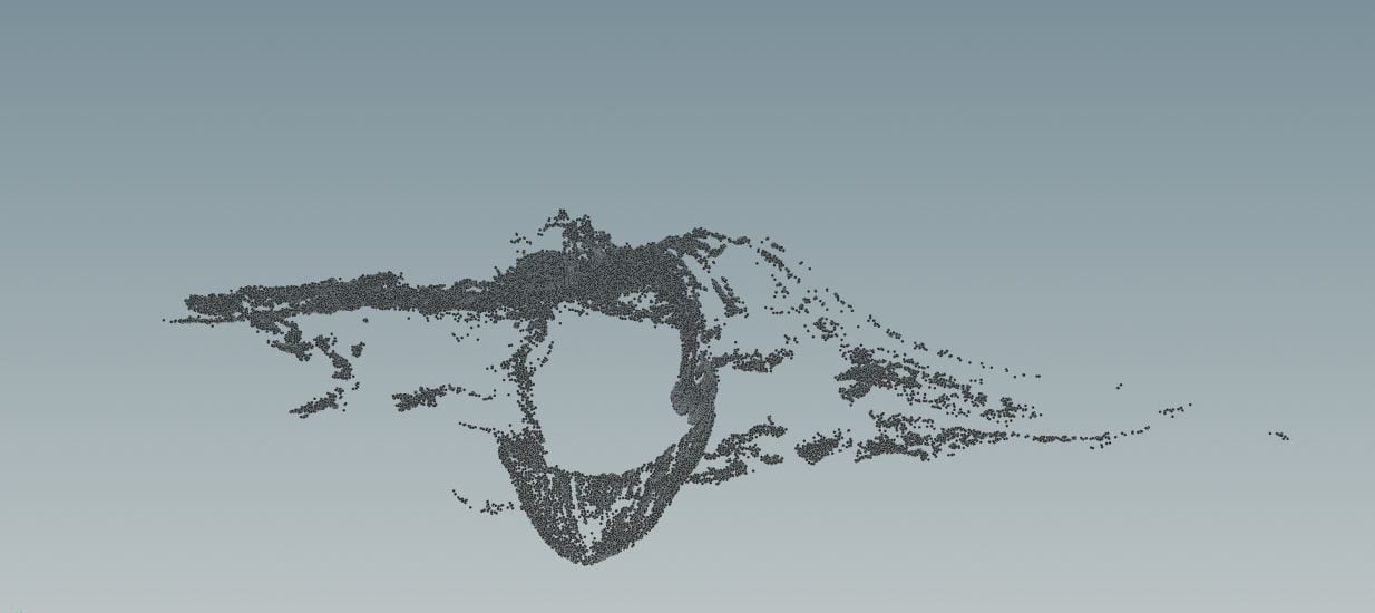
Our whitewater source now we have added the POPVOP.
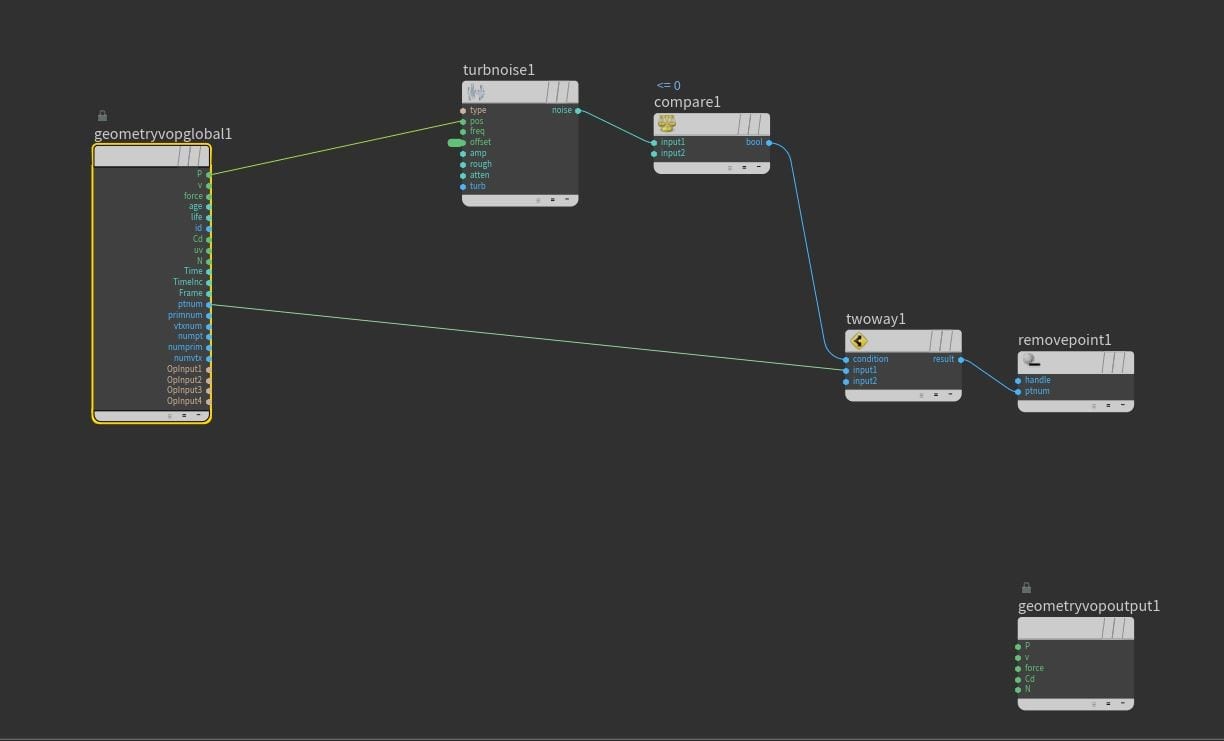
The interior of our POPVOP.
Lastly Giesen recommends dropping down a Cache node before the output Null as Houdini does not atomically store the whitewater source in the cache meaning every time you want to play your simulation the source will have to re-simulate.
Whitewater_SIM
whitewater Emitter
The most important parameter in this node is the Constant Birth Rate as this will effect the particle count of you whitewater with more particles being generated the higher the value. It is worth doing a number of flip books experimenting with this value as it will change depending on the motion of the boat and how big you want your splashes to be, for our simulation the default 100 is fine for now.
Next, in the shape tab of the WW Emitter we have a few parameters that will really effect the look of our whitewater. Firstly the shape itself will manipulate how the whitewater is distributed during a splash, like the Birth Rate it is important to do a few flip books to see which shape will look best for you, in this case we will use the cone. Also lower the Velocity Strength to reduce how far the points are spread and, because we want our points to spread from the bottom, change the Velocity Offset to 0 rather than the default 0.5. We also don’t want to stretch the velocity any further so reduce the Uniformity Scale to 1.
Thought our Whitewater Source was random enough by this point? Think again. Next we have the Noise tab of the Whitewater Emitter, toggle this on and we will add some further noise using the Sparse Convolution Noise Type increasing the Amplitude by at least double to give it some more influence.
Lastly, in the Attributes tab, we will edit the velocity settings of our Whitewater. Currently our particles are inheriting far too much velocity from the emission points making the splashes look over the top and unrealistic. This can be fixed by lowering both the Inherited and Radial velocities significantly to keep the particles closer together.
Collisions
At the moment our whitewater will just spray everywhere and not interact with our boat. This is not what we want, luckily it can be fixed very easily: If you head back to your GOL_Sim and copy the three nodes on the left (Static Object, Merge, and Static Solver) then you can simply paste these into the whitewater_sim in the same position and plug the Static Solver into the Merge node before the output. Remember to have the promote the Static Solver to the first input slot of the Merge and now your whitewater will collide with the boat collision geometry we created in the previous post.
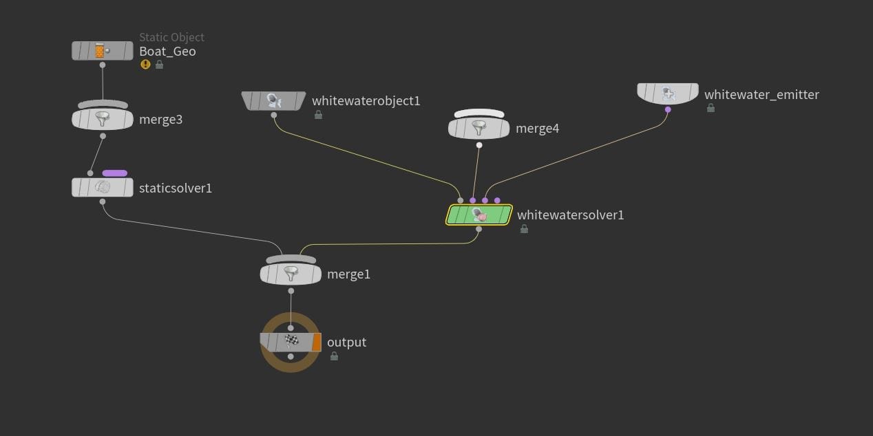
Our whitewater_sim with the collision geometry imported.
Whitewater SOlver
We covered many of the properties of the Whitewater Solver in part 2 of this series of posts, looking at the customisable factors of Foam, Bubbles and Spray so I won’t be explaining their various properties, only how to manipulate them ti get the desired look for our stormy scene.
Foam – One parameter we did not cover in part 2 was the depth, this will effect the thickness of our foam layer at the top of our water so we will increase it ever sos slightly for that extra foam. The current lifespan settings are fine as we are prioritising spray, just remember to toggle Preserve Foam to enable that clumping effect of groups of foam we already discussed.
In the Behaviour tab we have a number of settings we haven’t looked at previously, as a lot of these are inherited by the Spray we will take a closer look at these now. The Advection Strength effects how the velocity of the fluid will effect the foam and the default is fine for now, the Depth Scale however needs reducing significantly to add some surface tension to our foam – this will, again, assist with that clumping effect enabled by the preserve foam. Also decrease the Variance and increase the Move Amount allowing the particles a bit more freedom to move to their calculated locations.
Lastly in the Foam tab we will be looking at the Depth Scale Lifetime Ramp. If you observe any reference footage you will see that in such a scene, when a splash is created, first the foam and spray stick together, then begin to break up ready to be vaporised. Using the Depth Scale parameter we have ensured they stick together at first; now, by creating a convex curve that starts at a very high value before quickly dropping and stagnating (as pictured below) we can prepare for this vaporising effect.
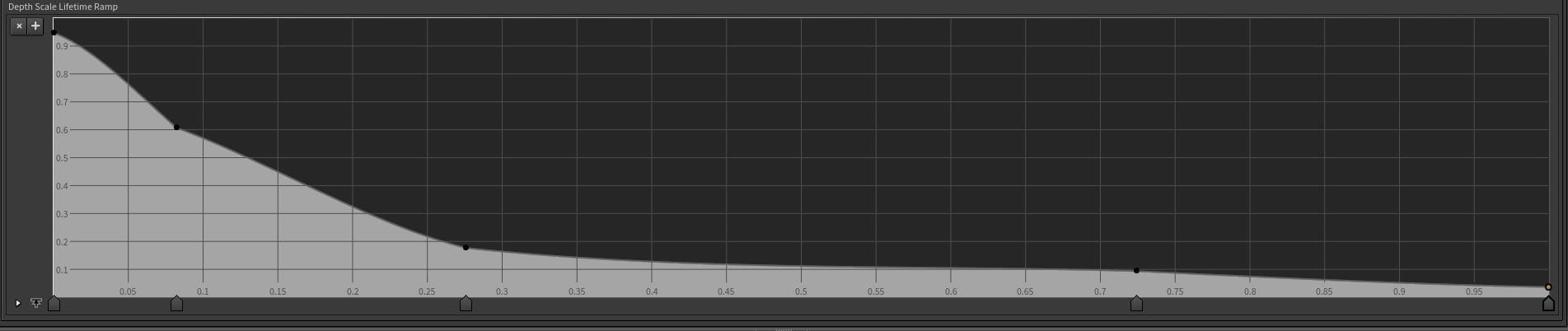
The Depth Scale Lifetime Ramp.
Spray – On the spray tab we have fewer options to manipulate, make sure to activate the drag so the particles do not fly too far in one direction and look unnatural, but lower the value so it doesn’t look too simulated.
Bubbles – As we are not going to be able to see through our ocean surface we will disable the bubbles as we won’t be able to see them anyway and it will slow down simulation times significantly.
Further Collisions
Now we have tweaked our networks create a flipbook of the simulation to see what the particles will look like and what kind of effect the splash will create. In Giesen’s simulation it appears some of the particles created by the splash are landing on top of the boat and, as we only created collision geometry for the hull, going through where the cabin of the boat will be; we therefore must revisit our collision geometry and add a bit more.
We only want to create new collision geometry for the whitewater however, not the GOL_sim, so we will need to duplicate many of the nodes in our Boat_Geometry network. First copy and paste the four nodes below the first Poly Extrude node (Collision Source 1, Attribute Create 1, the File Cache, and the VBD Null), as well as the Transform Node that moved the boat down, the Transform Pieces node and the Assemble, Blast and Rest nodes. Then set up this new path by connecting the output of the new Rest node with the left input of the new Transform Pieces, then the output of that into the new Transform node and the output of that into the input of the new Collision Source.
To add the cabin to the collision geometry just go into your blast node and select the cabin primitives using the little arrow next to the Group parameter and pressing the enter key.
Now, to update the connection in your whitewater_sim, go into the Static Object node and change the SOP Path to the Attribute Create of the new path you just made and the Proxy Volume to the new VDB null. This is all, I imagine, quite difficult to follow without visual aids so I will include a number of screenshots here to show all the new paths and what your Boat_Geometry network should look like now.
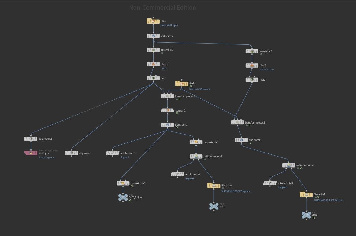
What your Boat_Geometry network should be looking like now.
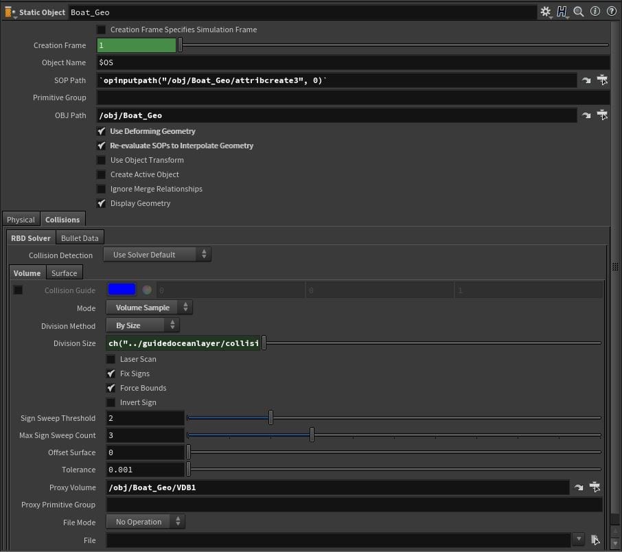
The updated SOP Path and Proxy Volume.
Custom Forces
Vapouriser
In order to vaporise our spray we will need to add some more noise and some wind to our scene, fortunately the Whitewater Solver’s second input allows us to add particle forces. To do this we will use another VOP network so drop down a POPVOP Node and connect it to the second input of the solver. Firstly in this VOP add a divide node connecting the Age of the Geometry VOP Global to input 1 and the Life to input 2 in order to create a normalised version of the Age parameter – this will define the amplitude of our noise. Next drop down a Curl Noise, plugging the Div output of the Divide node into the Amp (amplitude) input. Drop a Ramp Parameter node between these two to give us some extra control, making sure the Ramp Type is set to Spline not RGB.
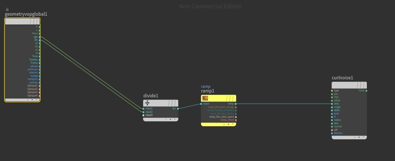
Our VOP Network in its current state.
Now if we go up one step out of the VOP and into the whitewater_sim we can edit the ramp from here. We want the vaporisation effect not to start immediately so point one’s position should be increased a bit with the value left on 0. Giesen uses 0.1 meaning that when the normalised Age parameter equals 0.1 the vaporisation will begin. This is because point 2 has a value of 1. However, we wan’t to speed up the amount of time it takes for our vaporisation to happen so decrease the position of point 2 to around 0.3. Now when our particles normalised age reaches 0.1 the vaporisation will begin until the normalised age reaches 0.3 when they have been fully vaporised.
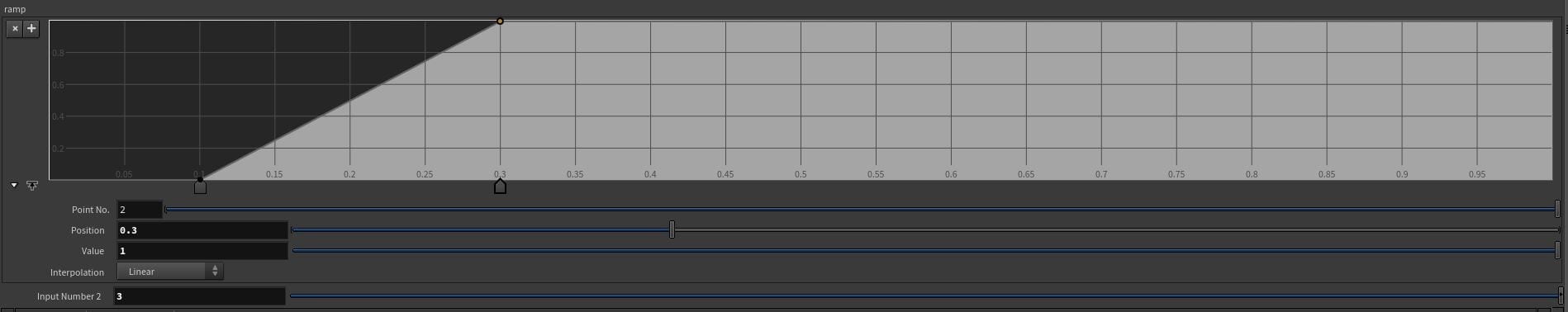
Our Normalised Age ramp.
We now need to add some additional values back within our VOP network so jump back in and connect the Force parameter of the Geometry VOP Global to the Force of the output. We want to add the force so drop an Add node in this connection and plug the Noise output of the Curl Noise into input 2 so this is added as well.
Our noise needs some tweaking first however, firstly we want to use Sparse Convolution Noise instead of Perlin Noise again, also we need the position to be defined by the Geometry VOP Global so plug the Position parameter of into the Pos input of the Curl Noise. At the moment the particles won’t be spread out very much as the frequency isn’t particularly high so increase this a bit just to pronounce the effect a little more. For experimenting purposes we should also drop a Multiply node between the ramp and the noise nodes so instead of having to keep changing the values of our noise, we can just change one in the multiplier. Promote the Input 2 parameter and then this can done just by clicking on the VOP Network in our whitewater_sim. Make sure your vaporiser POPVOP is only effecting the spray by toggling on the Group option and typing “spray” into the field then do a few flipbooks experimenting with different values in the multiplier, using your reference videos as a guide, and hopefully you should find a value that works for your purposes.
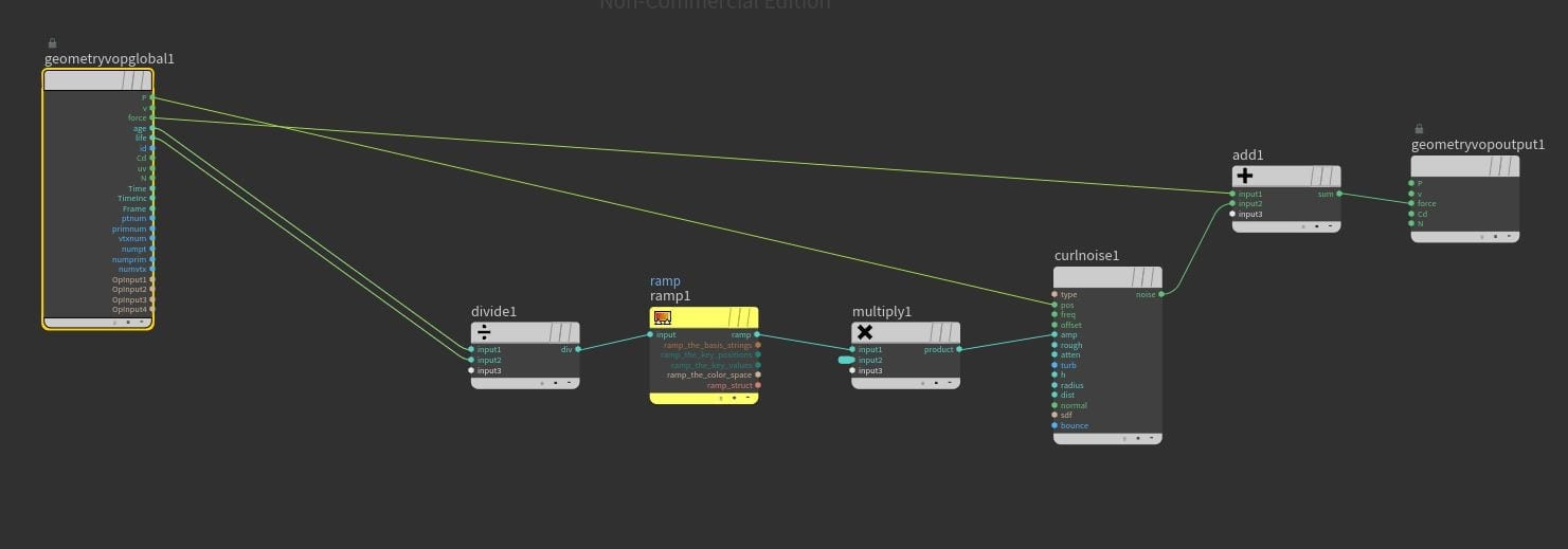
Our VOP network in it’s final state.

A frame of my flipbook after adding the vaporiser.
Custom Wind
According to Giesen the best way to add realistic custom wind to our simulation is to build it ourselves. To do this we’ll need a new geometry network so return to the Object layer and drop down a Geometry node. We don’t need the File node so get rid of it and drop down a box making sure it’s big enough to cover the area your boat will be sailing in – this Box will serve as a bounding box for our wind tunnel.
Next add a Volume node and connect it to the Box output, changing the Rank to Vector and set the name to “vel’ (velocity). We need the volume to be broken up into a lot of smaller ones in order to simulate our wind so change the Uniform Sampling to “By Size” and increase the Div Size a little bit so it will still iterate fast, but be detailed enough to appear realistic.
To give our wind some velocity the next node in our chain should be a Velocity Volume (make sure chain is plugged into the left input). The wind will always be there so toggle on Constant Velocity, our boat is moving forwards more or less along the x axis against the wind so make sure this number is the biggest and is also a negative, decrease the y value to give the wind a subtle uplift, and also add a subtle push to the z axis (Giesen settles on -2, 0.2, 0.5).
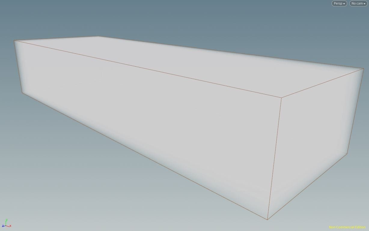
Without an appropriate method of visualisation you wind just looks like a big block of fog.
As per usual we need to add some noise to our wind otherwise it’ll look too uniform, this doesn’t require adding any more nodes, simply toggle on the Curl Noise tab in the Velocity Volume. At the moment it is hard to see what the effect of all this is as at the moment we only have a big block of fog in out viewport, to see the effect of the wind drop down a Volume Trail node (connecting it to the chain via the Velocity Volume in the right input), as well as another new Volume node with an Initial Volume of 1, 1, 0 and a Uniform Sampling Divs of 50. Connect this to the output of your original Box and then add a Scatter node with Total Force Count of 11,000 between the new Volume and the Volume trail meaning that we have two paths in our network as pictured below.
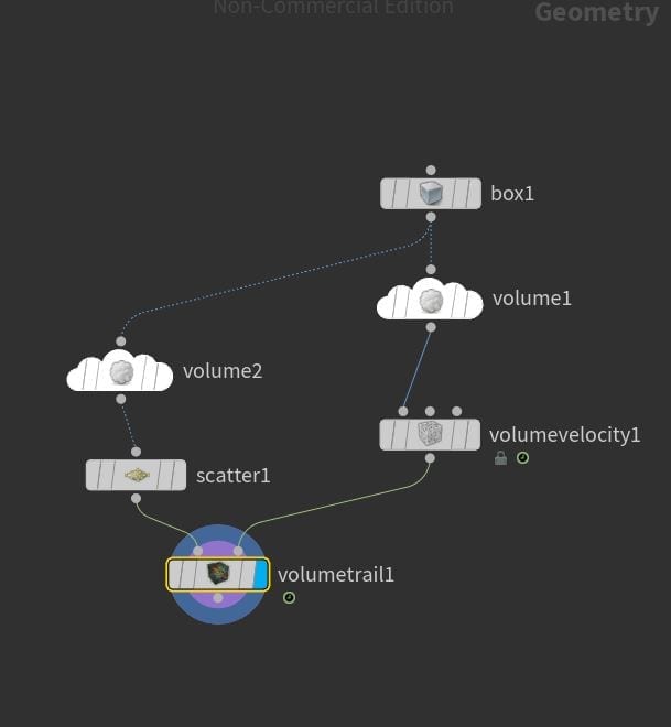
Your Wind network with visualisation capabilities added.
This new path in the network will not effect our simulation, it is just to visualise how points would be effected within our wind tunnel; now, if we set the view flag to our Volume Trail, we will see the effects of our wind.
Now we have a much more appropriate representation of our wind.
Now we can see the effects of our wind, we can edit the Curl Noise of the Velocity Volume to create the desired effect. Significantly increase the Swirl Size to really break up the uniformity of the wind as well as the Pulse Length and our wind should be ready to be applied to our particles.
To do this add a Null at the end of the chain (connected to the Velocity Volume output as we don’t want our visualisation) then head over to the whitewater_sim network. To import our wind into our simulation we can use the very useful POP Advect By Volumes node. As this also needs to be plugged into the second input of the solver, drop down a Merge node and plug both POP nodes into it. Set the Group of the POP Advect to “spray” again and then make sure the node is bringing in your wind SOP by setting the SOP to the Null we just created in the Wind network, making sure that Export Relative Path is toggled on so it is put in the context of our simulation. Confusingly, we don’t want to have Treat As Wind toggled on as we don’t want to add Air Resistance or drag, only Force Scale which we will increase along with Velocity Scale so our wind will influence our scene a bit more.
To see the effects of our wind do another flipbook and compare the results to your previous books before the wind was added. At this point, if your wind is too strong, too weak, or blowing in the wrong direction you can go back into the Wind network and tweak some of the parameters we have just set.
A screenshot of my flipbook with our added custom wind.
SOP Solver
Our whitewater still isn’t quite sticking together just after it’s emission as much as it should so, to fix this, we will use a SOP Solver. Giesen quickly glosses over exactly the function of a SOP Solver just highlighting that it is time dependent so I consulted the SideFX website that explains: “The SOP Solver DOP lets the DOP simulation use a SOP Network or chain of SOPs to evolve an object’s geometry over time.” (SideFX, 2018), essentially over a time period we can manipulate what an object looks like – which is exactly what we want.
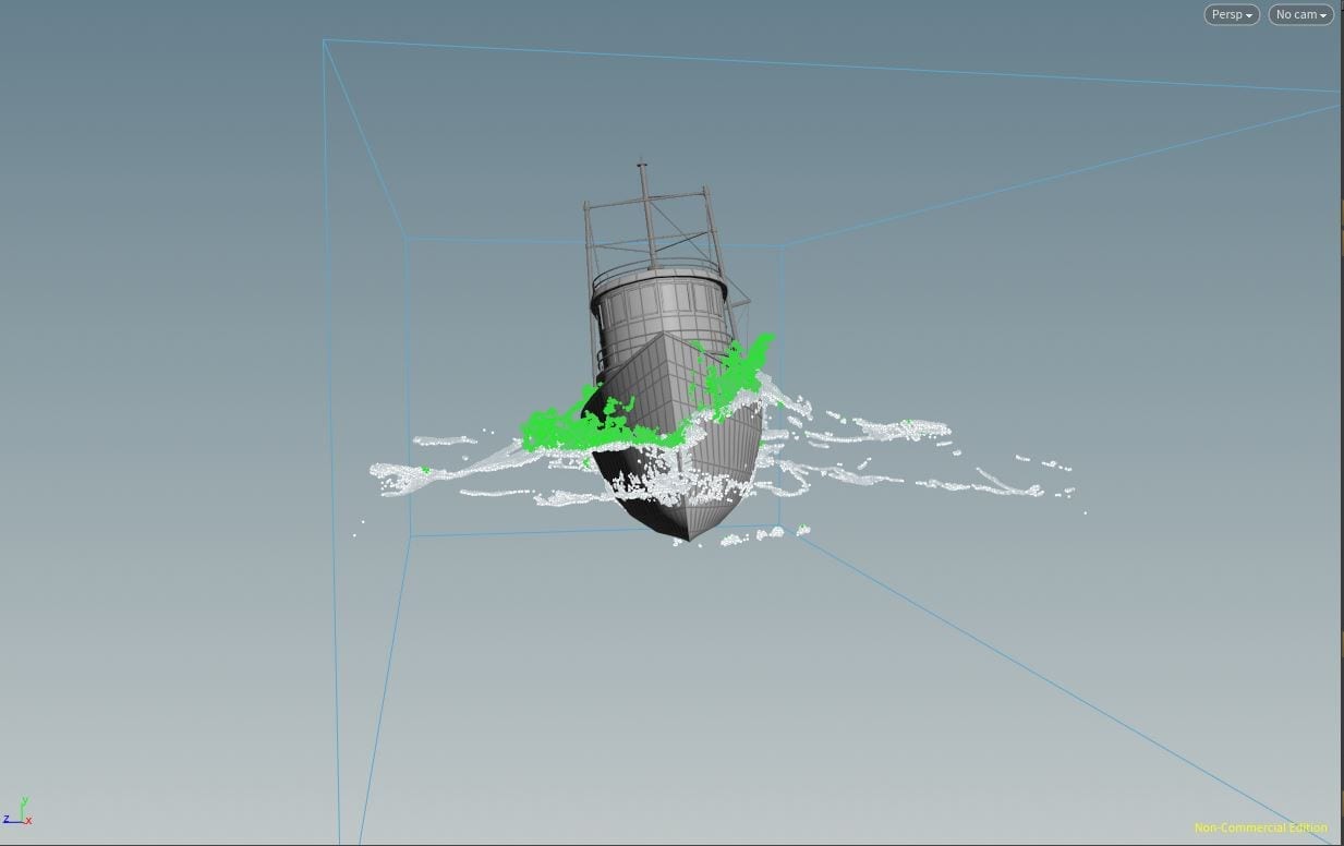
The SOP Solver connects to the fourth input of the Whitewater Solver so connect it up and then double click on the SOP Solver to jump into it. To get the particles to stay together we need to make sure they have the same velocity, to do this we will mesh together all the particles in the SOP solver to create one velocity that we can then reapply and blend into to the particles at the beginning of their emission, stopping them from spreading out.
Firstly we need to isolate the spray so connect a Blast node to the bottom of the DOP_Geometry node, set the group field to “spray”, make sure the Group Type is set to Points and toggle delete non-selected. To mesh together the points drop down a Particle Fluid Surface node, you may recognise this from the GOL_Fluid and GOL_Fluid_Extended as these types of nodes are also used to mesh together the FLIP Fluid particles to create our ocean surface. Plug the Blast into the the left input and if you visualise it you will see the particles have been meshed together. To improve the mesh for our velocity transfer, first lower the Particle Separation and change the Output, Convert To parameter to just Surface Polygons. The only attribute we want to transfer is velocity which is represented by the lowercase letter “v” so make sure the only letter in the Transfer Attributes field is v. Also, to decrease sim time, decrease the influence scale to 2 as 3 isn’t necessary for such a subtle change.
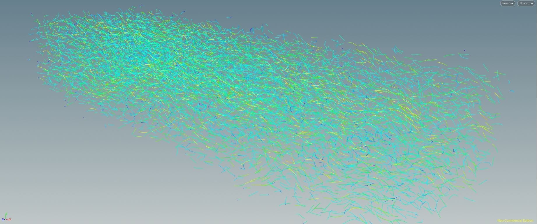
To check that this is working, in your viewport toggle the display velocity option and all the little blue trail lines in a section of the mesh should be pointing in the same direction. If this is the case then we now need to transfer this new velocity back to the whitewater particles so add an Attribute Transfer node to the bottom of the chain so that the original DOP_Geometry node is plugged into the left input and the Particle Fluid Surface in the right. Set the Points field to the letter v as we only want to transfer the velocity and untick the Primitives option as we only want to transfer point data.
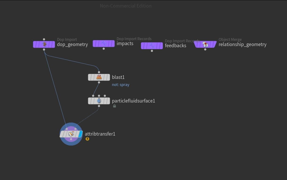
The interior of my SOP Solver.
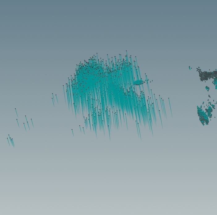
Notice how all the velocity indicators are pointing in the same direction.
To make sure this doesn’t slow down our simulation too much, in the Conditions tab set the Distance Threshold and the Blend Width to 1, and change the Kernel Function to Blinn Model. Unfortunately, at the moment, we are just overriding the original particle velocity with our own rather than blending in the new one, this is not what we want. To fix this we will use another Point VOP (first input DOP_Geometry, second input Attribute Transfer) and we will create a similar set of conditions to our previous VOP network to ensure the velocity is blended in and only blended in during the first few frames of emission.
As the velocity is what we’ll be blending connect the v output of the Geometry VOP Global to the v input of the Output node. Add a Divide node and set it up the same as before to create the normalised age as well as a Ramp, again set up the same as before. This time however connect the Ramp output to the Value input of a Fit node and promote the Destination Max parameter so we can control it from the SOP Solver. In our vaporiser POP VOP we used an add node next, however we want to blend in our velocity so drop a Mix node between the Global and Output nodes with the output of the Fix node connected to the Mix’s Bias input. At the moment we are not blending our original velocity with anything however so create an Import Point Attribute node with the Attribute set to v which, as we know, represents velocity and the Input set to Second Input (remember we plugged the Attribute Transfer into the second input of the Point VOP?). Now, if you plug the Result into the Input 2 of the Mix our velocity will be blended based on the Ramp and the Fit parameters.
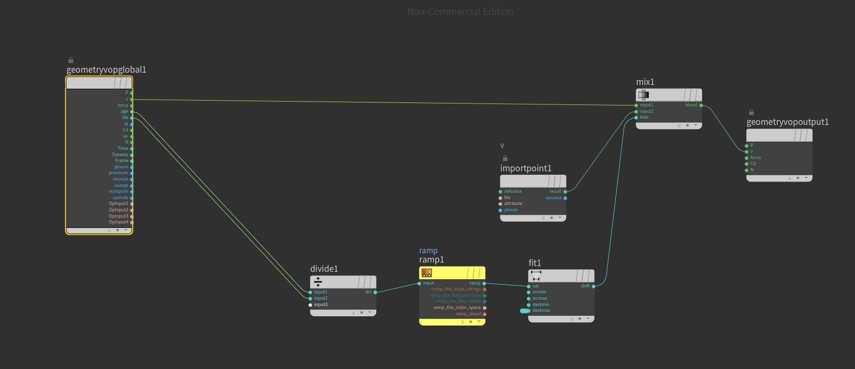
This time we are using a Mix node to blend in our velocity.
Now we need to set up our ramp, if you remember before in our vaporiser we had it so that the vaporising happens towards the end of our normalised age. Well this time we only want the effect of our VOP at the very beginning of emission so bring point 1 to a value of 1 at the very beginning of our ramp timeframe (position 0), and point 2 to a value of 0 so we have a decline in the effect over time. Set the position of point 2 to about 0.35 so our spray doesn’t clump for too long. Giesen adds a third point between the original two at the approximate normalised age 0.2 bringing the value down slightly to make the ramp convex. Now the velocity blend will only happen in the first few frames of the emissions’ life but the effect is a little too strong so reduce the promoted Destination Max value significantly to reduce this.
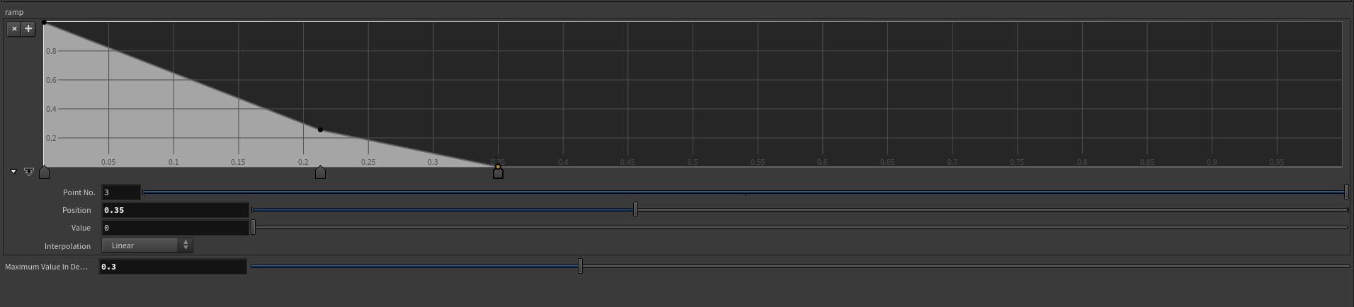
A ramp dictating the effect of our VOP network.
We are done with our SOP solver now, if we jump back to the whitewater_sim we can flipbook our updated simulation. If you compare the previous flipbook with the new one you will see the effects of our SOP solver. I’m sure you will agree they are very subtle differences, however it is these subtle differences that trick the eye of the viewer into believing what they are watching is real.
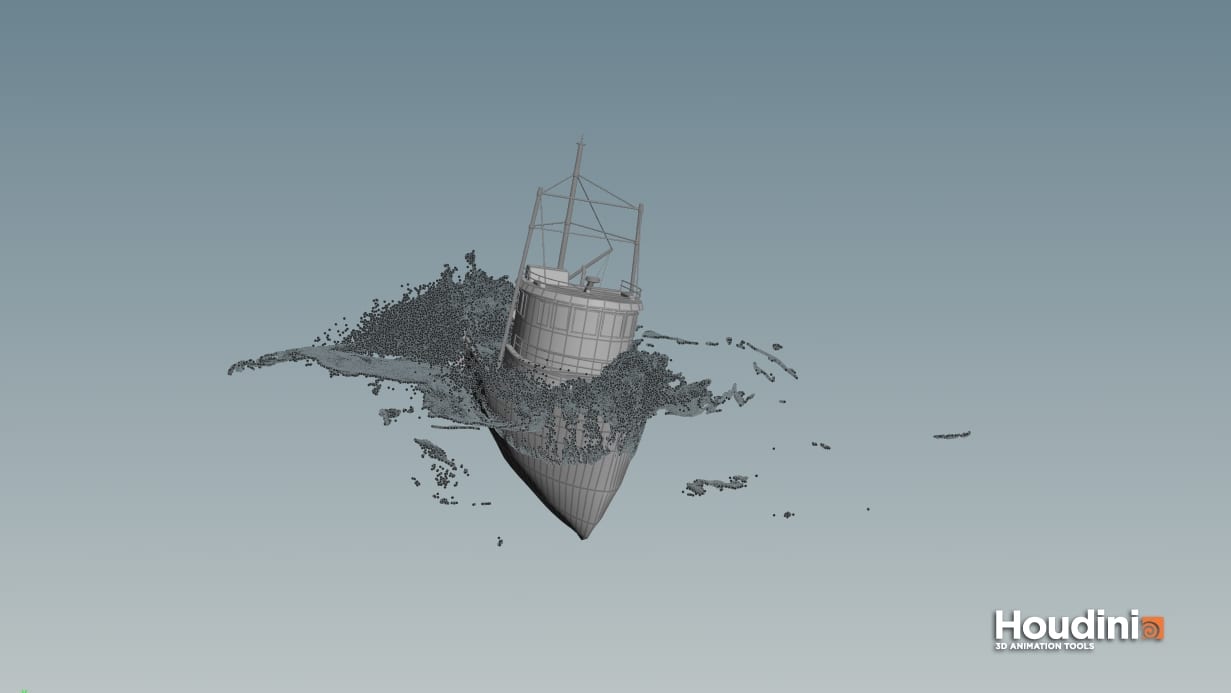
A screenshot of my my final flipbook using the cached whitewater.
Caching our Whitewater
We’re now done creating our whitewater and are nearly ready to cache it out. Firstly though we need to increase the amount of whitewater particles generated as currently it isn’t nearly enough, to do this we need to increase the Const. Birth Rate of our Whitewater Emitter. The amount to increase this to differs based on the specs of your machine and how much it can handle, mostly in terms of RAM, Giesen has a 64gb machine and so chose a value of 10,000 however for lower spec machines he provides a series of lowered values more appropriate for the reduced memory. I have 32gb of RAM in my machine so i used half this, with a value of 5000 my machine took 2 and a half hours to cache out my whitewater so adjust your Birth Rate accordingly.
Before we cache out our whitewater, to reduce sim time, we will first cache out our whitewater_source using the File Cache node that’s already there. Make sure the path is set correctly and the whole frame range will be cached then hit Save To Disk – to import the cache back in create a new File node and plug it into the network like we have done previously.
As we have done previously make sure Allow Caching is toggled off in the Whitewater Object node on your Sim take so all of your memory isn’t consumed, as well as disabling any Cache nodes you’ve added for fast iteration in the viewport.
To cache our whitewater simulation we will need a ROP Output Driver, jump into your whitewater_import network and drop one down and connect it to the output of the Import_Whitewater node. Confirm the path and frame range as per usual and make sure the Render With Take is set to Sim not Main then save the cache to your disk. To bring this back in, drop down a File node and locate your cached file, however for now leave it out of the network chain as the file should be about 80gb.
End of part 5
We still have one more step before we can start the materials and render process. In the next part, to add one final layer of detail, we’re going to add some mist to our simulation that will really sell that this really is a stormy ocean scene.
REFERENCES
- Pluralsight (2017) Houdini: Intermediate Ocean FX. Available from: https://app.pluralsight.com/library/courses/houdini-intermediate-ocean-fx/ [accessed 28 October 2018].
- SideFX (2018) SOP Solver Dynamics Node. Toronto: Side Effects Software Inc. Available from http://www.sidefx.com/docs/houdini/nodes/dop/sopsolver.html [accessed 28 October 2018].