

Introduction
Before we can apply the materials to our ocean and render the final video there is one more addition we need to make. To add one final layer of realism to our shot we will create a mist layer.
Generating Mist
Thankfully we do not have to create our mist from scratch, in the Particle Fluids tab of the shelf there is a button labeled Mist, similar to the whitewater, to create it, click on the shelf button then select your Guided Ocean Layer in the GOL_sim then, with your mouse over the viewport, press Enter. If we look at our Object layer we will see three new networks have been generated, just like with the whitewater we have the mist_sim, mist_import and mist_source. These nodes serve the same purpose as their whitewater counterparts so I won’t cover them in detail, in shorthand the source generates the particles that get solved by the sim which is then imported by the import network and is what we will render at the end.
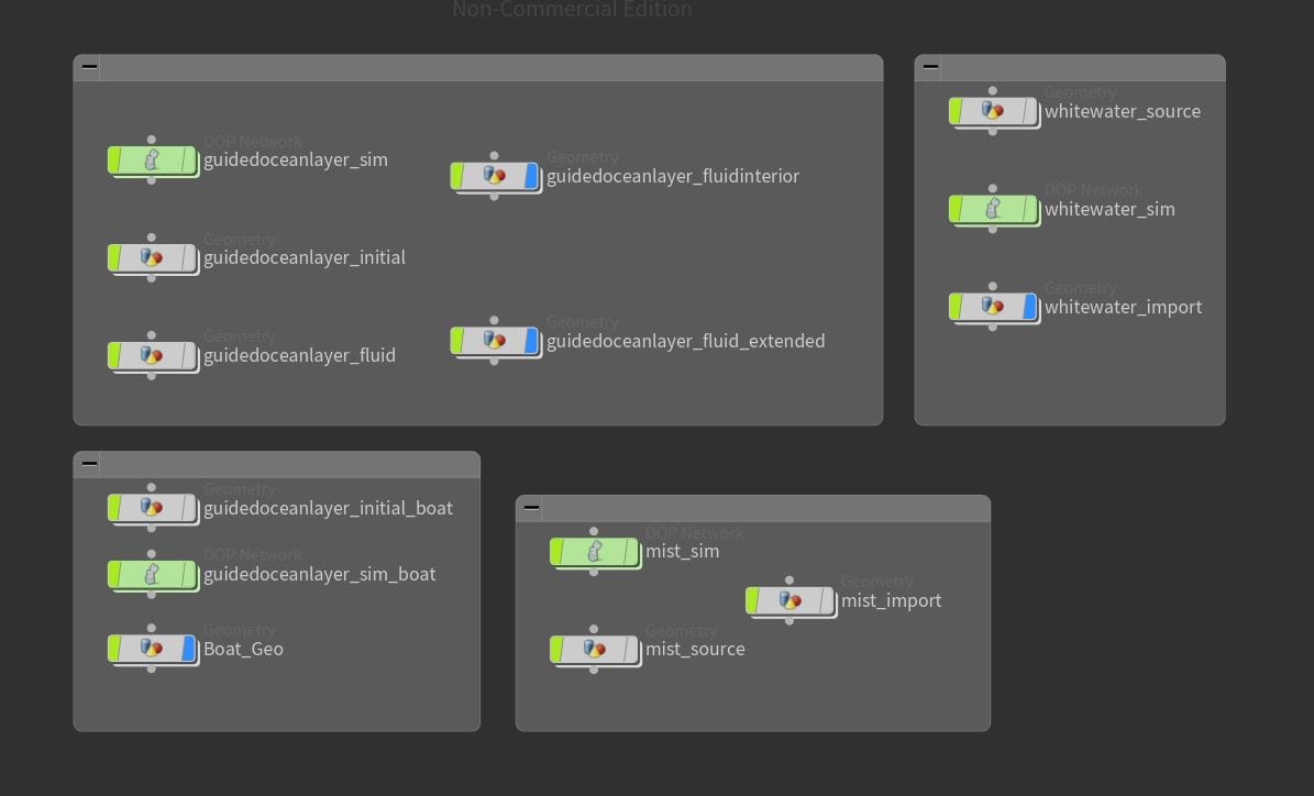
Our object layer after we use the Mist shelf tool.
Whitewater Source
A few tweaks need to be made in this network as we want a subtle layer of mist not only generated from the FLIP Fluid but also by the whitewater spray itself. Firstly, to speed up our simulation, untick Reseed Compressed Fluid; then, to make the whitewater generate mist as well, drop down an Object Merge (disconnected from the chain for now) and set Object 1 to the whitewater cache we created at the beginning of the previous part. Also, because we use our own File nodes to re-import our caches the path of the Object Merge at the top of the chain needs to be updated to our FLIP cache in the GOL_Fluid.
If you MMB on the whitewater Object Merge you will see we have about 8 million points (depending on the birth rate you used) being brought in by our WW cache, this is far too many for such a subtle layer so connect a Delete node to the bottom of the Object Merge. Within the Delete set the Entity to be deleted to Points and we want the Operation to be Delete By Range, then set the Select_Of_ to be 9, 10. What this means is that out of every 10 points 9 will be deleted. Now you should have only 10% of your WW points remaining which is much more appropriate for our mist. Now we need to add the whitewater particles to our chain so drop a Merge node below the Mist Source and connect the Delete to the top.
Rather than creating emission particles like the whitewater_source our mist_source is created a dense volume that will actually plug into a Pyro Solver in the mist_sim. While pyro simulations are something we will be covering in a whole separate series of posts there will be some overlap here as Houdini uses pyro physics when creating mist from the shelf. If you put the display flag on the Create Density Volume you will see this in the viewport.
We want the most mist to be generated by the faster moving spray particles so to do this we will create another ramp. Firstly drop down a Point Wrangle between your Delete and Merge node. To isolate the faster particles we first need to calculate the total velocity, to do this use the VEXpression:
f@vTotal = length(v@v);
To use a ramp our values have to be between 0 and 1 (remember we had to use the normalised age in our VOP networks?) so we will add a second expression called a lookup. Create a new line in the VEXpression field and add:
f@vTotal = length(v@v);
f@lookup = fit(@vTotal,0,10,0,1);
So what this line does is it takes our original velocity which currently has a maximum value of 10 and scales it down so that instead of being between 0 and 10 it is between 0 and 1. Lastly we need to create our ramp, we want the ramp to effect our particle density and we will use the lookup as the ramp attribute so the last line of VEX you need to add is:
f@vTotal = length(v@v);
f@lookup = fit(@vTotal,0,10,0,1);
f@density = chramp(“ramp”, @lookup);
Now if you hit the button next to the VEXpression field labeled Create Parameters your ramp will be created at the bottom of the Point Wrangle.
The greater our particle’s density the more mist will be generated, as we mentioned previously we want the faster whitewater particles to generate lots of mist and our slow ones to generate next to none. The ramp represents our fit velocity running from 0 – 1 along our x axis and density along the y so we need to create an inclining gradient. Giesen uses these parameters for his ramp: P1 (pos = 0.2, val = 0), P2 (pos= 0.5, val = 1) meaning that the slowest 20% of particles won’t generate any mist and the fastest 50% will generate the maximum amount.
As we have just create a specific density attribute for our whitewater locate the Create Density Attrib node in the chain and move it so it is between the Mist Source and the Merge, otherwise it will overwrite the density we have have just assigned to our whitewater particles also lower the Value significantly otherwise the emission will be too dense.
The last step in our mist_source is to drop down another Point Wrangle, this time just below your Mist Source, to remove any particles unnecessarily generating mist below the surface of our water. To do this use the VEXpression:
if (@P.y < -0.5)
removepoint (0, @ptnum);
If you have the display flag set to the Point Wrangle or below you will immediately see a few points be deleted from the bottom of the viewport.
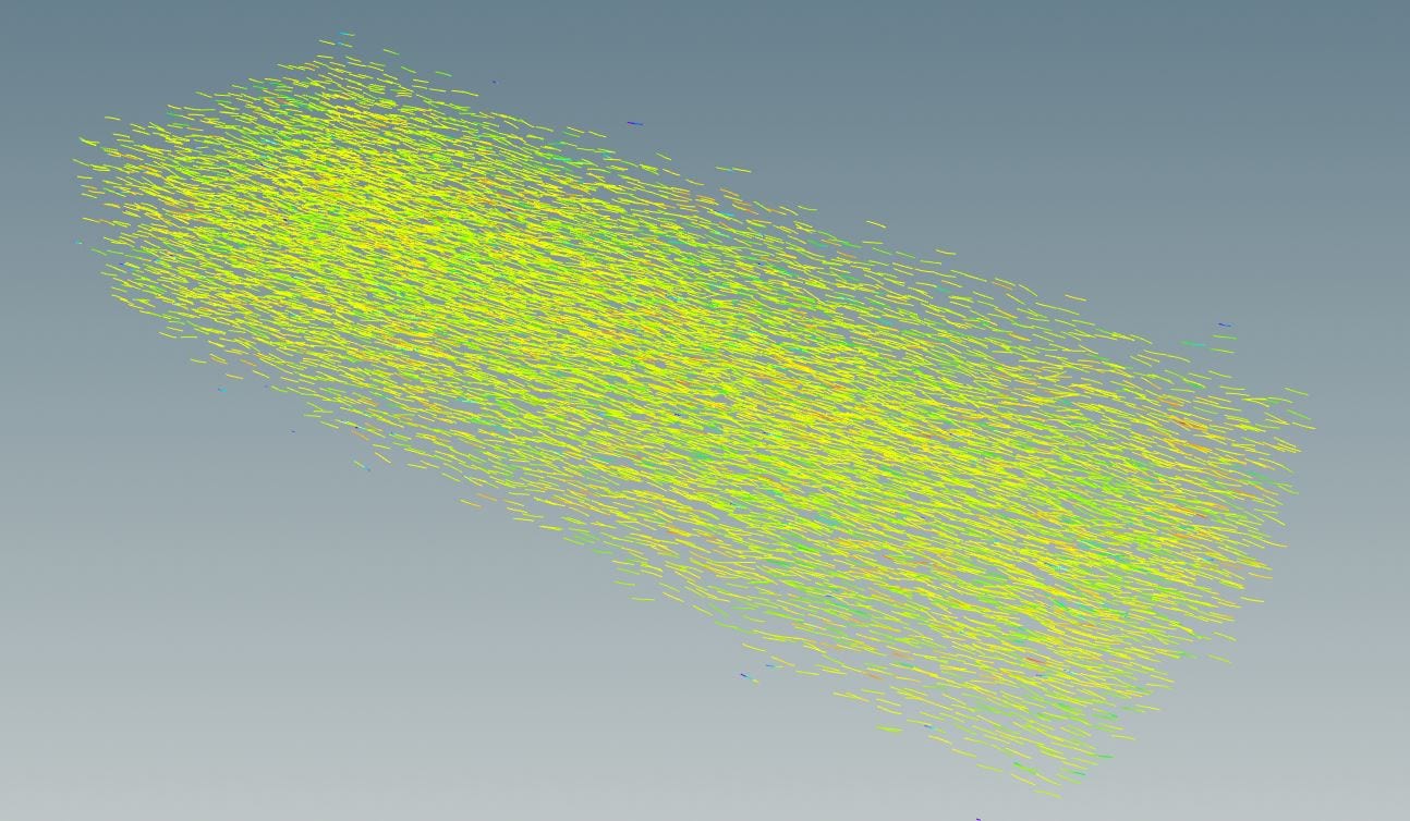
Now if you display the Create Density Volume you will see what our mist density looks like at the moment, the density should be thicker around the bow of the boat as this is where the particles are moving fastest. Most of the parameters in this node are fine to begin with however in this case we actually want to disable Noise – we have plenty already. Also, in the Stamp Points tab lower the Sample Distance so it only effects points that are a bit closer together, but increase the Point Sample Threshold just to smooth this effect out.
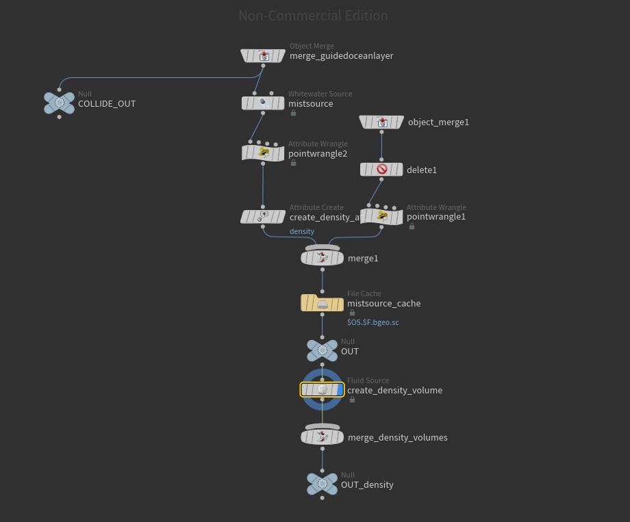
Our final mist_source network.
Our mist_source is now complete, one issue you may notice however is that if we try and play our timeline our sim speed has been reduced significantly, this is because the source is having to import two already pretty heavy caches. To increase sim speed we will cache out our mist_source using the Mist Source Cache (File Cache) already provided and then import it back in using a File node placed above the Out Null in the chain.
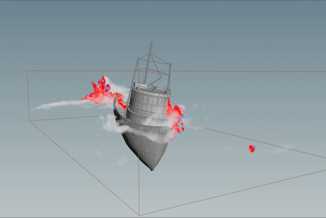
A visualisation of the density of our mist particles. In thicker areas more mist will be generated.
Mist_sim
For our purposes with the mist we will only be using the pyro, not the advection particles so the first thing you can do in you mist_sim is delete the two nodes connected to the fourth input of the Pyro Solver.
Currently the resolution of our sim is being halved so the first step is to delete the multiplier of the Division Size of our Pyro node so that now the Division Size should be 0.06.
Next we have the Resize Container, this is essentially a bounding box that, in this case, dictates where mist can and can’t be generated. In pyro simulation this is a lot simpler as generally the fire begins at one point however with our ocean we have waves generating foam all across our viewport and spray firing wildly so this node requires some tweaking to compensate. To do this change the Tracking Object from a DOP to a SOP and then locate the mist source cache File Node in the mist_source network. Now our bounding box will track to the mist source.
We also want to reduce the velocity of our source just a little bit so in the Source Volume on the far right of the network (source_density_from_mist_source) reduce the Scale Velocity parameter to about 0.1.
Now we can tweak our Pyro Solver. Firstly we want to give our mist some motion but we want it to sink rather than rise so increase the Buoyancy Life but make sure the Buoyancy Dir is set to a negative value in the y direction. The Combustion tab can be skipped in this case as we are working with mist not smoke.
In the shape tab increase your Dissipation parameter to make sure the mist fades away quickly as well as the Disturbance. The Confinement parameter is fine how it is but disable the turbulence as, after this, we will create our own wind for the mist. Scroll down and in the Dissipation tab disable the control field so it acts on our whole density field also, in the Disturbance tab, Giesen recommends linking the Block Size to the Division Size of our Pyro node so no anomalies are generated, to do this copy the Division Size Parameter and then “Paste Relative Reference” in the Block Size.
The rest of the Pyro Solver is fine how it is, that was a very brief look at quite an important node, unfortunately we are only dealing with fluid simulations at this point however we will revisit the Pyro Solver later when I look at pyro simulations in the second half of this blog.
The last two steps in the mist_sim is to import our boat collision geometry. This can be copy paster over from the whitewater_sim like we did before, just paste it over and plug it into the Merge node above the output, remember to promote the Static Solver to being the first input or the Relationship is set to Mutual. Finally drop a Gravity node after the Merge just to really emphasise the sinking effect of our mist.
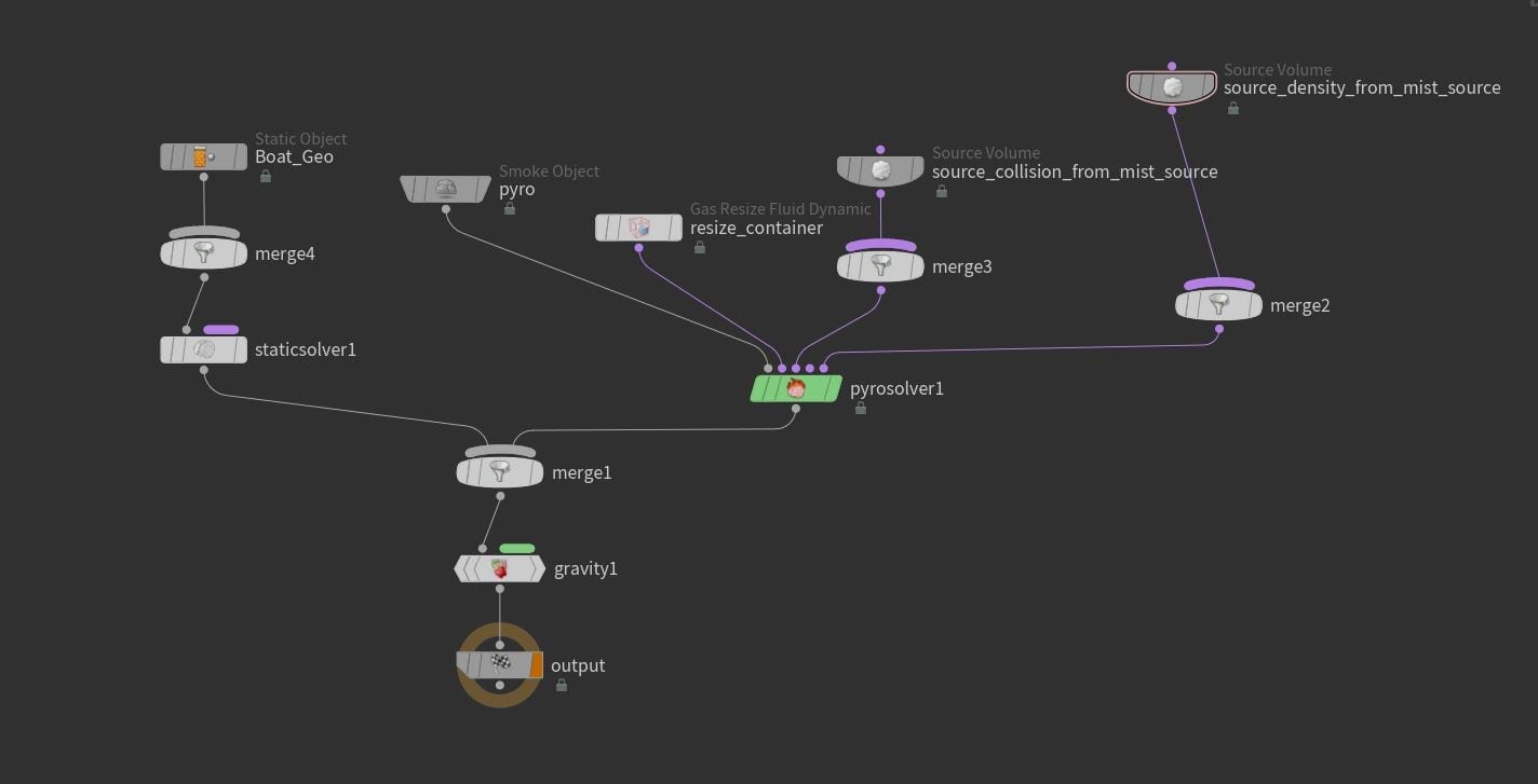
The mist_sim network with the boat collision geometry added.
More Custom Wind
Our mist wind will be similar to the one we used for our whitewater_sim but with a few tweaks so duplicate and rename the network then dive into your wind_mist.
We don’t want quite such a random look for our mist wind so, in the Volume Velocity, reduce the scale of the Curl Noise significantly; if you have your display flag set on the Volume Trail this should already look at lot calmer and more uniform. To further increase this effect increase the Pulse Length and our noise will move a lot slower.
Your wind should look a little calmer with the reduced Curl Noise.
Now with these changes made hop back into the mist_sim and drop down a Source Volume node and set the path to the OUT Null of our wind_mist (again with export relative path enabled). We don’t want to import the Volume or Temperature attributes of our wind so set the scale of both to 0 and in the Volume Operation tab set the Source Volume and Temperature to None. We do however want to add a reduced version of our wind velocity to set the Scale Velocity to around 0.3 and set the Velocity in Volume Operation to Add. To add this node to your network connect it to the Merge node connected to the last input on the Pyro Solver – now your custom wind will effect the mist.
The final Cache
We are almost done with the simulation section of creating our shot all that’s left to do is cache out the mist. As we have done before to conserve memory jump to your sim take and disable Allow Caching in the Pyro node Creation tab.
Next, jump into the mist_import and if you click on the Import Mist node and scroll down you will see it is important the geometry, we want to import the density so just replace the name in the field and set the object field to pyro.
Using the same process as in the whitewater_import drop down a ROP Output Drive connected to the output of the Import Mist, update the file path, make sure its baking with the sim take and rendering the frame range not just a single frame. Once the cache is done use a File node to import it back in as we have done previously.
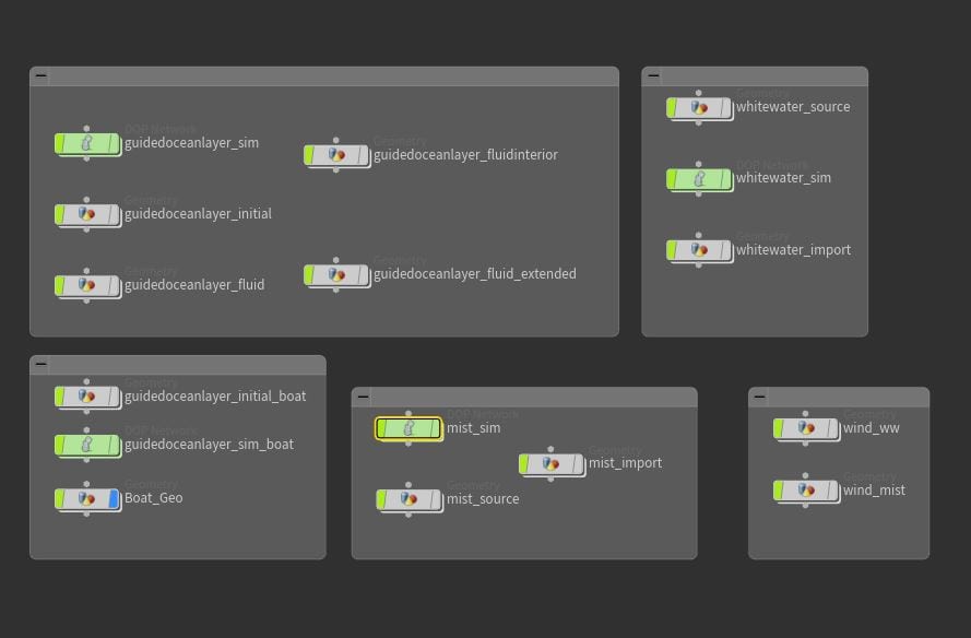
Our final object layer, I have used collapsable groups to keep my various networks tidy.
End of part 6
We are finally here, the simulation phase of our ocean shot is complete from here we just have to set up the lights, add materials to our ocean, set up the render nodes and then wait for the shot to be rendered. So we aren’t actually all that close to the end but there should only be one more post in this series before I can start creating my own shot using these posts as a guide.
REFERENCES
- Pluralsight (2017) Houdini: Intermediate Ocean FX. Available from: https://app.pluralsight.com/library/courses/houdini-intermediate-ocean-fx/ [accessed 29 October 2018].