
Introduction
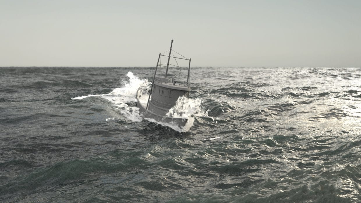
We’ve reached the final module and final blog post in this series of instructional guides on how to make a stormy ocean shot in Houdini. First we imported our boat and set up the FLIP tank and ocean displacement layer, then added the whitewater containing the foam and spray and lastly simulated an extra layer of mist to add a final layer of detail. All that’s left now is to set up our light and camera, apply and tweak our materials, and then set up the render nodes to export and composite our final sequence.
Shot set-up
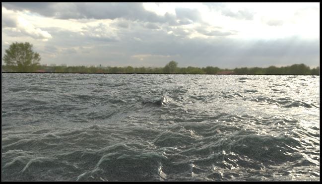
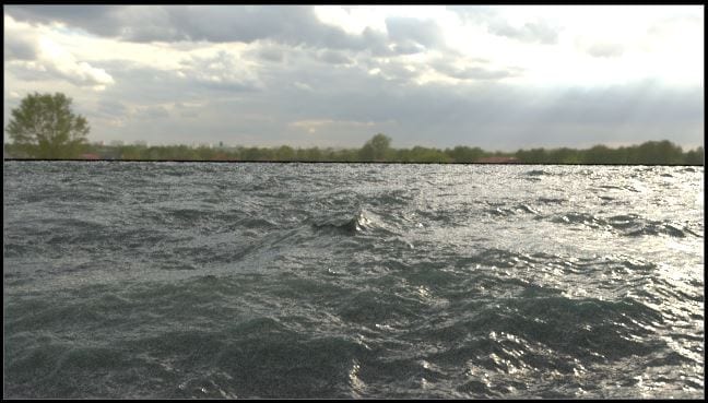
Before we can set up accurate materials we need to set up the scene. Firstly, drop down an Environment Light in your object layer and browse for an Environment Map. Giesen includes his own EM as part of the downloadable course files however for my final shot I will source my own, luckily many are available online for free, try to find as close an environment to a stormy ocean as possible, download it and load it in. Increase your light intensity to better light your shot and, to view your EM as part of your background toggle on Render Light Geometry and Clip To Positive Y Hemisphere so only the top half, above your horizon line, is used.
The displayed environment map.
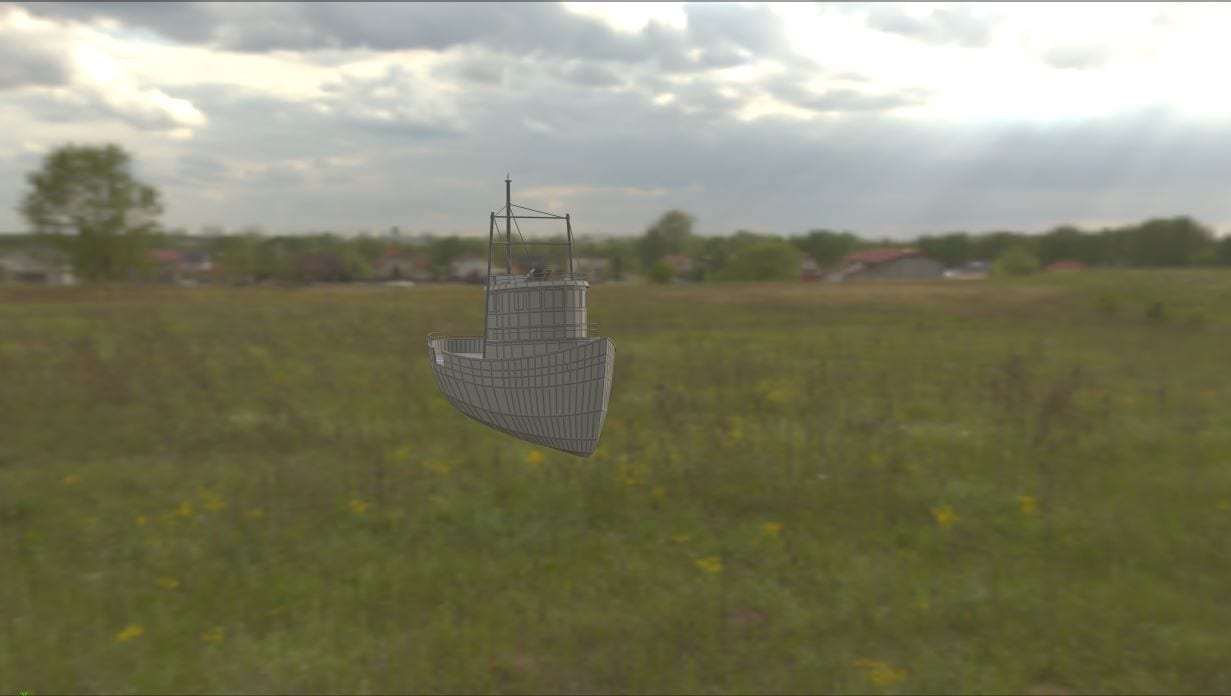
Next we need to make one final adjustment to the Boat_Geometry network so that the whole boat, not just the hull is rendered out. Duplicate the Transform Pieces and connected Transform node again, and connect the Transform above the Assemble nodes’ output to the first input of our copied Transform Pieces. Add a Null labeled “Render” after this with the render flag set to it so Houdini will always render this from our Boat_Geometry.
Lastly add a camera to your scene using the tab in the top right, Giesen provides a camera with the project files however the only difference between this and a regular camera is some animated movement. If you wish to create an animated camera for your scene that is up to you, it can be done very simply using keyframes.
Extending and Meshing the Sim Area
Extending the GOL_Fluid_Extended
We need to mesh our particles together to form the surface of our ocean if we want to apply materials to it. Dive into the GOL_Fluid_Extended and you may see some of your nodes have error markers – if not that’s fine too it is still worth taking this step – this is because the Object Merge is trying to import the compressed cache and simulate it. We baked out our compressed cache a couple modules ago so drop down a File node, locate the compressed cache and then replace the Object Merge with your File node.
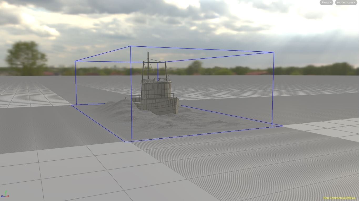
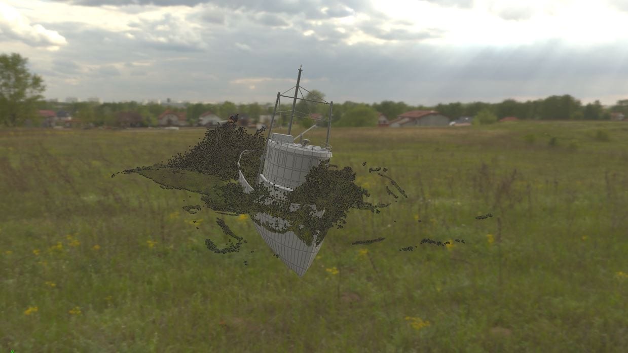
First, before we mesh our ocean together we need to extended the ocean layer as currently it is only a small square. Click on the Surface Preview node in the GOL_Fluid_Extended and head over to the Regions tab. Make sure the display flag is set to this node, at the moment the waves should only be surrounding our boat in a small circle, to fix this change the Shape parameter to rectangle, however now the waves look really cut off at the edges of our preview which will look very odd in the meshing so increase the Flatten Distance so you have a bit of padding to work with. We also have some quite big waves so increase the Max Height to at least 4 – more if you’ve got some really big waves.
Next we need to toggle on Pad Bounds which well let us extrude the area of displacement for our ocean. Set the Extrude Polygons to Along Each Axis so we have a bit more control and then increase the Extrude Distance significantly. If your camera shows the horizon line, like mine does, then you are looking to create an ocean that looks infinite so you need a big value, Giesen uses 1500.
Our extended displacement grid.
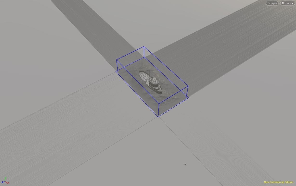
To make sure we aren’t generating loads of unnecessary geometry behind your camera let’s also toggle on the Camera option and set the path to the camera we just set up. Currently you won’t see anything as the default Z Near and Far are set to only mesh between one and two meters, we want the meshing to start really close to our camera so reduce the Z Near to basically nothing and then we need to have at least 1500 + however far our camera is from the centre in the Z Far so put a generously large number there to give yourself some leeway like 2000.
The mesh should look really weird at the moment, that’s because it’s meshing extending at an angle with very low divisions. To fix this, firstly increase the Extrude Divisions to at least a few 100, then we need to scale up the Window X and Window Y values – just scale these up until you have a decent overlap all the way around your frame.
Now we have our camera tab on, only the displacement in front of the frame will be generated.
We need to link our parameters to the Particle Fluid Surface so scroll up in the preview and change the Rebuild SDF to Adaptive then, using the Copy Parameter/Paste Relative Reference method link all the parameters we’ve just set in the Surface Preview to the Particle Fluid Surface.
Meshing Our Particle Fluid Surface
Now we can tweak the Surfacing tab of our Particle Fluid Surface. A lot of these values are fine already, the first three parameters control the resolution and should all be fine how they are, the Particle Separation is linked to that of your sim network so if you increased that of testing make sure you lower it again so our mesh is detailed. To add add some detail in the particles themselves reduce the Droplet Scale and the Erosion Scale to get rid of any seams around the edge of our simulation area. In the filtering tab we can further edit the look of our mesh, by default they are all toggled off. We just want to enable the Dilate and Erode options, both of which are fine with their default values.
Tweaking the mask
In part 4 I mentioned that this workflow works by creating a small FLIP Tank for our Boat to interact with and seamlessly blends it with a displacement based ocean layer, to finalise this process we need to cache out our Mask and Spectra. Currently though, if we display our Ocean Evaluate we will see two things, the blue section looks very odd and not much like waves (this is because of low resolution) and the red section looks very tall and out of place in comparison (because there is too much displacement).
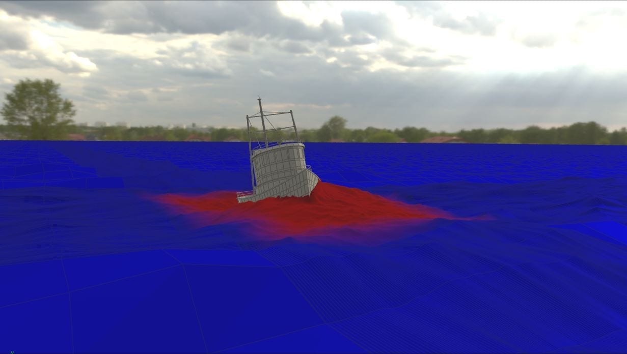
Our displayed Ocean Evaluate node – it needs some tweaking.
To fix this we will look at the two nodes controlling our masks, the Particle Fluid Mask and the High Frequency Mask. The first one makes sure that the displacement is only happening right up to the edge of our sim area with a feather so they merge nicely and isn’t what is causing our issues. The High Frequency Mask, however, needs some adjustment. The purpose of the HFM is to take the high frequency detail of our displacement layer and add it to the simulation so it looks like there’s no difference between the two.
To lower the small hill of waves we have building around our boat go into the Spectrum tab of the HFM and make sure Remove Non-Spectral Waves is enabled; because we have added custom waves the algorithm cannot figure out what waves are below the set Amplitude Resolution above so we have to do it here manually.
Fixing UV Tiling Anomalies
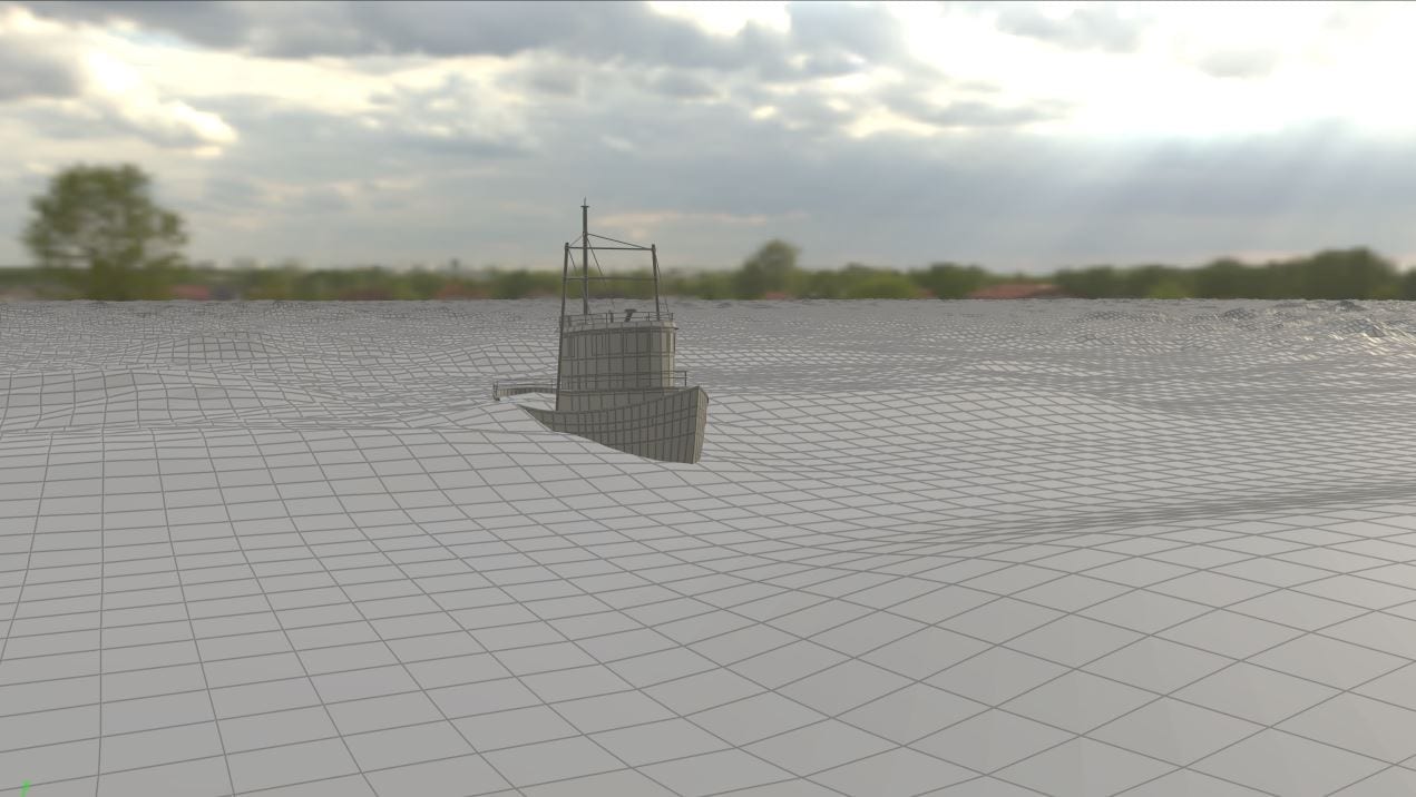
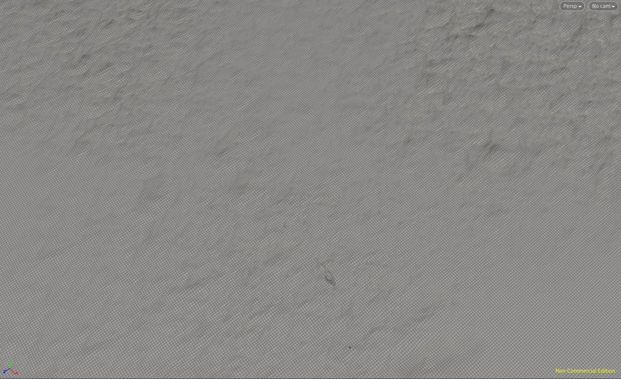
We need to view what our displacement will look like in our extended area as well now so head over to the GOL_Initial and duplicate the Grid Preview and Ocean Evaluate nodes. To increase the grid area, break the connections in the Size parameters and change the values to 1500 in each direction. Currently it should look really low resolution because the Rows and Columns don’t have a high enough value so break that connection as well and increase them both until the waves are looking a little more realistic.
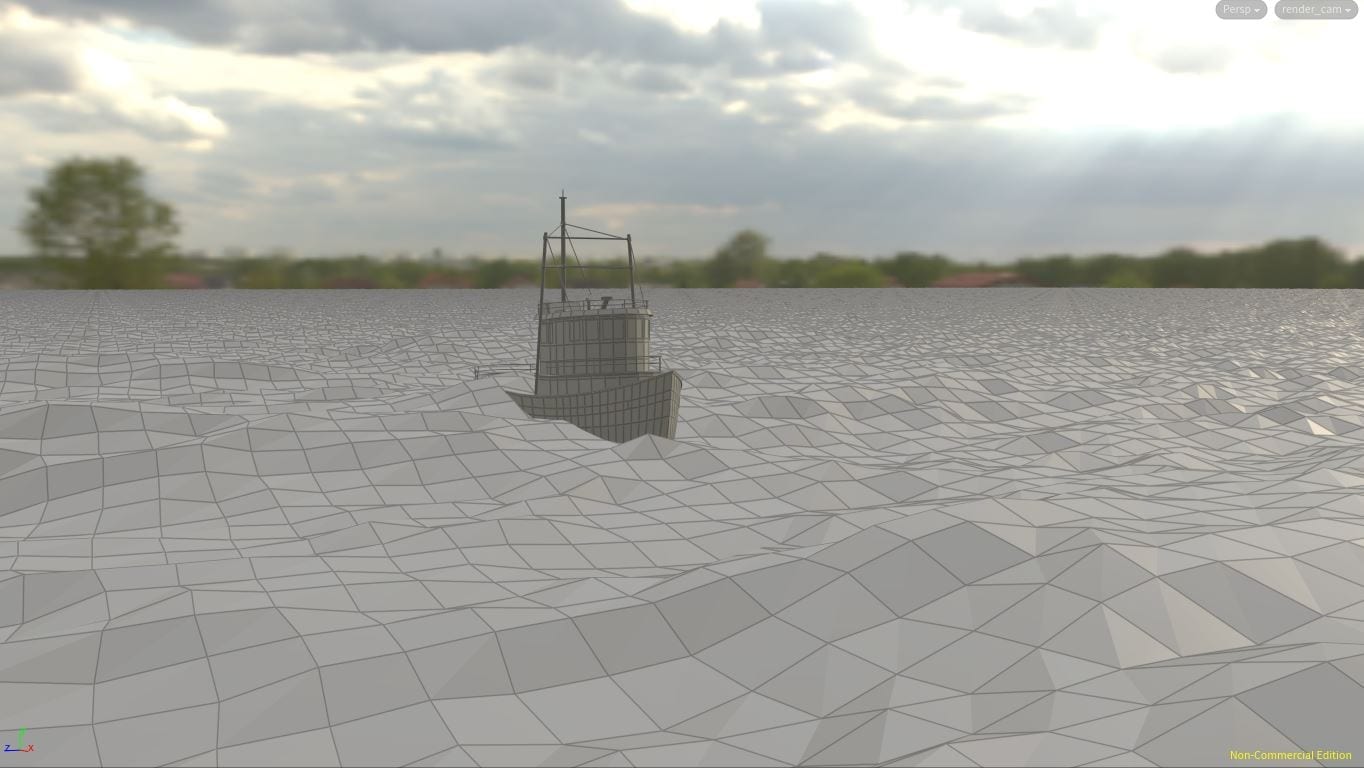
Our low resolution extended grid.
Immediately you should see the issue we’re going to encounter when rendering, in the left and right corners of our ocean there is a very obviously repeating pattern. We discussed the concept of UV tiling in part 2 of this series and the balance between grid size and tile size to trick the viewer into not noticing the tiling. To do this we will isolate the foreground (which already looks how we want) from the background (which we want to edit).
Unfortunately this is the only part of the module Giesen does not explain in detail on how to construct from scratch, instead he provides some nodes in the project files for us to copy into our own network alongside a short description of the purpose of each, however I will attempt to explain them here. The chain we need to build for this isolation is as follows Grid > Scatter > Delete > Split > 2 Ocean Spectrums (the split has two outputs, an Ocean Spectrum attached to each).
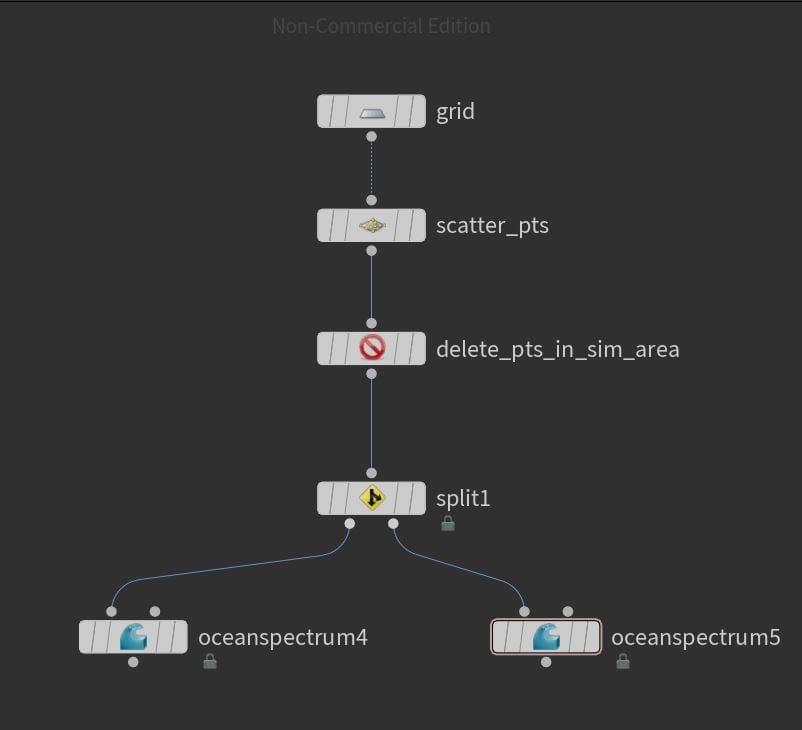
The background isolation chain.
The way this chain works is: we start with a large grid that covers the size of our ocean, then points are scattered all across this grid using the Scatter node. In the Delete node all the points in the foreground are deleted using the Bounding Volume method of deletion – essentially creating a volume in the centre of our simulation in which all the points are deleted, leaving only those outside remaining. The split node breaks these remaining points into two groups, to do this Giesen uses the expression:
0-‘npoints(opinputpath(“.”, 0))’:2
Attached to each of the split outputs is an Ocean Spectrum set up similar to in part 3 so they “roughly match with our simulated area but with more variance”. To then add these two new spectra to the ocean duplicate the Merge Spectra node, it should already have the original spectrum and the custom waves attached, just add the two new Ocean Spectrum nodes to the input at the top then connect the output to the right input of the new Ocean Evaluate and you should see in the viewport that your UV tiling issue is fixed.
The last step in this process to make sure the original Ocean Spectrum is not being rendered underneath new ones in that background area to save on calculation time. To do this we will use the Wave Instancing feature. Copy your original Ocean Spectrum node and disconnect the original from the new Merge Spectra, replacing it with the duplicated Ocean Spectrum. We will create one point to use as our instancing point for the wave instancing and then fade it out around the edges, to do this drop down an Add node and toggle on Point 0. It should already be in the centre so just connect it up to the left input of your Ocean Spectrum and you will notice a change already in the viewport.
Our instancing radius is currently far too low so only our custom waves are visible in the foreground.
This is obviously not the desired effect so jump into your Ocean Spectrum node Wave Instancing tab and we will tweak the settings. We need a much bigger Radius to cover the whole simulation area so increase it to 160 and make sure none of your parameters have any Variance or it will edit the actual Ocean Spectrum settings. You can disable both the Rotation and the Offset as we won’t be using either of these, in the Amplitude however increase the value to 1 otherwise the settings from the Ocean Spectrum will be reduced. If you zoom out you can see the effect this is having, we have 3 large circles, each of which corresponding to one of the ocean spectrums, we could do with a little smoother of a fade though so reduce the Rolloff to about 2.
The three large circles: 1 in the foreground, 2 in the background.
The last step before we bake out our mask and spectra is to add a little more detail to our Ocean Spectrum. The spectrum we just duplicated and added the instancing to is our new main spectrum so increase the Resolution Exponent to 10, we won’t be simulating anymore so detail is more of a priority than sim time.
This often can create some undesirable noise in your ocean, luckily it can be fixed by toggling on Remap Amplitude in the Amplitude tab and tweaking the ramp. Increase the Max Remap Resolution to 9 and modify the ramp so it dips down in the middle – it is simpler to show you want I mean than write it so here is a screen capture of my ramp to show you what I mean.
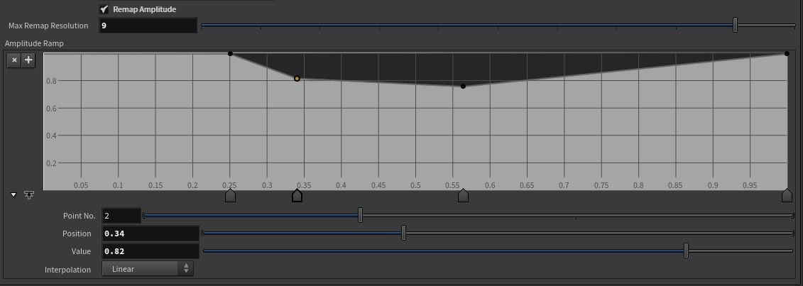
My resolution ramp.
Our ocean would really benefit from some extra noise to break up any last bits of uniformity, not necessarily in the sim area but around the edges so toggle on Add Noise in the Mask tab. We don’t want it to be obvious we are generating extra noise so set the Size values so they are not the same. Make sure the Direction is set the same as it is in the Wind tab so our waves are going in the same direction and reduce the Roughness significantly so we get nice smooth waves. Lower the Speed and increase the Pulse Length to get some nice slow waves and set the Offset values to 15, 0, 2 so that the simulated area is not being effected as much. Lastly decrease the Input Range and increase the Output Range so our noise only has a little influence and isn’t overpowering our original spectrum settings.
Baking The Mask and the Spectra
With all these tweaks made we are ready to bake out our Mask and Spectra. In our GOL_Fluid_Extended we need to update the connection in out Import Spectra node as we duplicated the Merge Spectra so edit the path in there so our new Merge is what is being imported (with Export Relative Path toggled on as usual). Now we are ready to bake, update the paths in the File Cache nodes if you wish then just hit Save To Disk. I recommend doing the Bake Spectra first as it only has to do 1 frame whereas the Mask has to do the entire range.
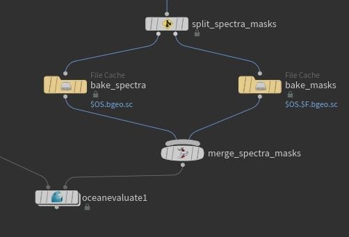
The two File Caches for the Mask and Spectra.
Materials
setting up the Ocean Volume
Time to head into the GOL_FluidInterior which currently looks quite friendly compared to some of our 25+ node networks. By default the Object Merge is importing the render Null from out GOL_Fluid which only covers the sim area so update this to the same Null in the GOL_Fluid_Extended.
We want our ocean to have some depth, even though our ocean surface won’t be especially see through it will still add to that extra layer of detail we’re going for, so drop down an Extrude Volume node below the Object Merge. Currently the volume is flat though so we need to apply our displacement, to both the GOL_Fluid_Extended and the GOL_FluidInterior. If you click on your GOL_FluidInterior and navigate to the Render Tab you will see the material is currently set to the Uniform Volume material, this is not what we want.
To change this swap over to the “Mat” (materials) layer and delete the Uniform Volume material, then click the Tools button > Show Tool Palette and locate the Ocean Volume in the Liquids group, to add it to your Materials layer just drag and drop it. We need to link a lot of the parameters in the Ocean Volume to those in the Ocean Surface so locate that material (it should have been created automatically in your Mat layer) and link all the parameters from Spectrum Geometry to Time using the Copy Parameter/Paste Relative Reference technique.
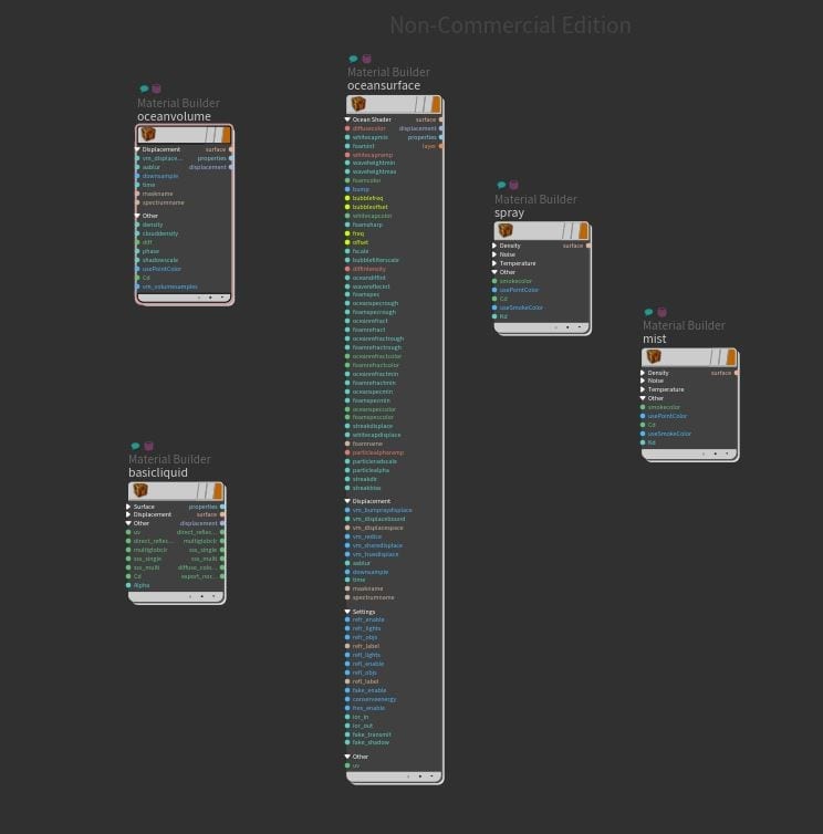
Our materials layer.
We now need to assign our material so back on the object layer locate your GOL_FluidInterior and under the Render tab set the Material to Ocean Volume. Then make sure your GOL_Fluid_Extended is set to use the Ocean Surface material and, under the Sampling tab, make sure Geometry Velocity Blur is enabled.
Our First Test Renders
In order to see what we need to change we need to render a frame of our simulation so, in the Out layer, drop down our first Mantra node – this will be the node we use to render our ocean so name it accordingly. We always want to be using our set up camera so set that parameter. For now reduce the Sampling from 9 to 4 and the Reflect and Refract limits to 2, just while we are previewing our render. Make sure the Render Engine is set to PBR (Physically Based Rendering) and lastly, just again to speed up preview times, override the camera resolution to 1/2.
Rather than chance it letting Houdini work out what we want to render and what we don’t, head into the Objects tab and remove the asterisk from Candidate Objects. Instead we will force the GOL_Fluid_Extended and Gol_FluidInterior by selecting them in the Force Objects field.
Head back to the Mat layer and we will set up our Ocean Surface material. First thing to do is break the connections on the Spectrum and Mask Geometry and set the path to the Spectra and Mask we baked out earlier. Because our waves are pretty big we need to increase the displacement bound to at least 4 to compensate. Now you can click on the Render View tab, set the Mantra_Ocean node as your renderer and hit the Render button to see what a frame from our scene looks like as of now.
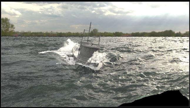
My rendered frame.
Tweaking the Ocean Shaders
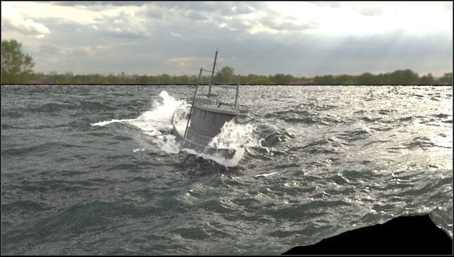
What’s immediately obvious from our rendered frame compared to our reference footage is there is far too much foam at the crest of our waves – we will fix this in the Ocean Shader tab. Firstly, because we have some pretty big waves, increase the Max Height to 3. To reduce the foam on our wave crests we need to lower the Whitecap Intensity, this will not effect our whitewater and as we have set up the foam we do want separately we can afford to reduce this value significantly. Lastly, before we do another render, in the Displacement tab, enable Add Bump To Ray Traced Displacement to add a really fine layer of extra detail to our Ocean Surface material at minimal render time cost. Now hit Render again to see the results.
Just by reducing the Whitecap Intensity our ocean already looks more realistic.
PREPPING the Whitewater for materials
Now we’ve set up the Ocean Surface material we need to sort out what the whitewater is going to look like. In our whitewater_import network we need to move the connection between the Import Whitewater node and the Attribute Wrangle over so it’s using the File node with our whitewater cache as the input instead. Otherwise every time we do a render it will have to first simulate what the whitewater should be doing in that frame, which we already waited (probably) hours for our computer to do earlier in the process.
The way our whitewater is rasterised as by taking all the points from our simulation and meshing them together in such a way that it looks like foam, we can tweak this process in the VolumeRasterizeParticles node at the bottom of our chain. Firstly though, to add a few more points to our whitewater, drop down a Point Replicate. Don’t connect it up yet though, the default point to point value is 100 meaning that we would be increasing the resolution by 100 times – essentially guaranteeing a crashed Houdini. Reduce this value to 3 then change to the Shape tab to make a few tweaks. We want to be using a the Line Shape not the Box as we only want to offset the points a little bit, also change the Velocity Stretch to Scaled but reduce that scale to 0.5 so the shape of our whitewater isn’t changed to significantly. Lastly, in the Attributes tab enable Copy Source Attributes otherwise the new points won’t have the attributes they need to be rasterised.
Now we can add this node between the Attribute Wrangle and VRP node in the chain and you will see our particle count increase in the viewport.
The increased point count on our whitewater.
The Spray material
Before we actually change any of our rasterising settings we will set up the material so we can see the effects of our modifications in the render view. In the Out layer lets duplicate our Mantra_Ocean node and rename it for our whitewater, remember to add the whitewater_import network to the Forced Objects, for now we will leave the ocean networks in there as well just for preview purposes, also add the Boat_Geometry network to this field for the same reason. Now fire off another render, this time using the Mantra_Whitewater.
There are two very obvious issues in our initial whitewater render.
There should be two very obvious issues in this render, firstly our whitewater looks like smoke, and secondly our ocean is being cut off in the bottom right corner (if you cannot see this jump to frame 130 and do another render, you will see what I mean). To fix the smoke issue head over to Materials layer and locate the Spray material. At the moment our spray is far too dense so reduce this value to 2 and reduce to the Shadow Density Multiplier to 0.015. If your render doesn’t update automatically do another one manually and you will our spray is looking a lot whiter but a little thick. We could still use a bit more brightness in our foam so increase the Smoke Intensity to 2.5 and then head back to the whitewater_import on the Obj layer where we will fix the rasterising and make our spray a bit thinner.
The Whitewater Rasteriser
The first step to fixing our rasterising is reducing the Particle Scale of our Rasteriser node significantly to about 0.15, this will make out whitewater far too thin but will provide a good starting point for this process. If we have a look in our VDB we will see the Voxel Scale is automatically linked to the simulation resolution, we need to lower this value further however so break the connection and reduce the value to 0.011. Now if we jump back to the Rasteriser we can increase the density scale to 40 and change the filter to Catmull-Rom, this means that we will have a lot of very small (as we lowered our P Scale) very dense particles making our foam a bit sharper. As we’ve lowered the Particle Scale we should also lower the Minimum Filter Size so make this about 0.5 and re-render.
Our whitewater is a lot more realistic already.
That’s it for our whitewater, the last step is just to create a render Null at the bottom of the chain with the render flag (ctrl-leftclick) set on it so we are neat in our workflow.
The Mist Material
The interior of the mist_import network is identical to that of the whitewater_import however, because of the nature of our mist, we do not need to rasterise it as we did not advect our particles in the Pyro Solver so just import the mist cache using a File node but don’t worry about adding it to the chain. Make sure the render flag is set to the File node, enable Geometry Velocity Blur on the network node itself, then locate the Mist shader in the materials layer.
The Mist shader is pretty fine how it is, only a couple tweaks need to be made, again increase the Smoke Intensity to 2.5 to increase the effect of our mist, but reduce the Smoke Density to 0.75 so it isn’t too thick and the Shadow Density Multiplier to 0.02 so it isn’t excessively dark. Add the mist_import network to your Mantra_Whitewater node (we will split it up later) and then hit render to see the results. As you can see it adds some transparency to the thinner parts of the mist and a nice, realistic looking, feather around the edges.
The mist layer is very subtle but adds another layer of detail.
Rendering and Compositing
We’re finally here, the very last step of creating our ocean scene, rendering out our final sequence. But first there’s one last issue to fix – the large black triangle in the bottom right of our simulation.
What are you triangle?
If we hop into the GOL_Fluid_Extended and display the Surface Preview you should see why the issue is being caused. Because we are using the Camera option to reduce the amount of displacement we have this cut off area at the bottom of our frame. Our extended displacement is already very high resolution so we cannot increase the Extrude Divisions even further, nor can we increase the scale of the Window X and Y. Unfortunately this means we will have to lose the Camera option so disable this. Now out extended displacement is covering the whole area, one befit of this is we can reduce our Extrude Divisions back down to 4 which is better for displacement and we will have to rely on Mantra not to worry about the displacement outside the frame. Click on the Particle Fluid Surface node and make sure the sane settings are applied in there – it is likely you will need to disable the camera again. If you were to re-render frame 130 again now you would see the triangle is gone and our displacement is working properly again.
Now the strange triangle has been removed.
Performance Tweaks
By doing this we have actually reduced our polygon count to about half which should actually reduce our calculation time significantly, killing two birds with one stone. Another way to further reduce this calculation time is in our GOL_FluidInterior > Extrude Volume, reduce the Depth from -1 to -0.2, while we do need some depth in our ocean surface, 0.2 metres will be plenty for our refraction purposes in such stormy weather.
Setting up the Render Layers
We already have two of our Mantra nodes half set up for the ocean and whitewater, quite a few of the settings need tweaking though for our final composition. Firstly toggle on Motion Blur and set the Geo Time Samples to 2, we have a lot of movement in our shot and it’s going to look very odd if all of our geometry is nice and crisp. We can now increase the Max Ray Samples again, Giesen says to use 5 but my render still looks a bit noisy and the default is 9 so for my final composition I will do a few test renders and find a value more appropriate for my purposes. The rest of the rendering options are fine, just remember to untoggle Override Camera Resolution or you’re going to get a very low resolution render.
Now all that’s left is to set up the Objects tab for each node. We need 4 Mantra nodes in total, one for the Boat_Geometry, GOL_Fluid_Extended and Interior, whitewater_import, and mist_import. In the Object tab we have the Forced Objects which is what we see in render, the Forced Matte which creates a transparent hole where that geometry should be and the Forced Matte which doesn’t generate visible geometry but still renders the refraction and shadows of the geometry. The Object tab should look as follows for each render node.
MANTRA OCEAN
Forced Object – GOL_Fluid_Extended
Forced Matte – Boat_Geometry
Forced Phantom – GOL_FluidInterior, whitewater_import, mist_import
Mantra Whitewater
Forced Object – whitewater_import
Forced Matte – GOL_FluidInterior, GOL_Fluid_Extended, Boat_Geometry
Forced Phantom – mist_import
Mantra Boat
Forced Object – Boat_Geometry
Forced Matte – GOL_Fluid_Extended
Forced Phantom – mist_import, whitewater_import, GOL_FluidInterior
Mantra MIST
Forced Object – mist_import
Forced Matte – GOL_Fluid_Extended, whitewater_import, GOL_FluidInterior, Boat_Geometry
The last thing we want to do before rendering is add some Extra Image Planes to our Mantra nodes. Find the tab and toggle on the Shading Depth and Combined Lighting so, in compositing we have the option to modify the reflection, refraction and intensities.
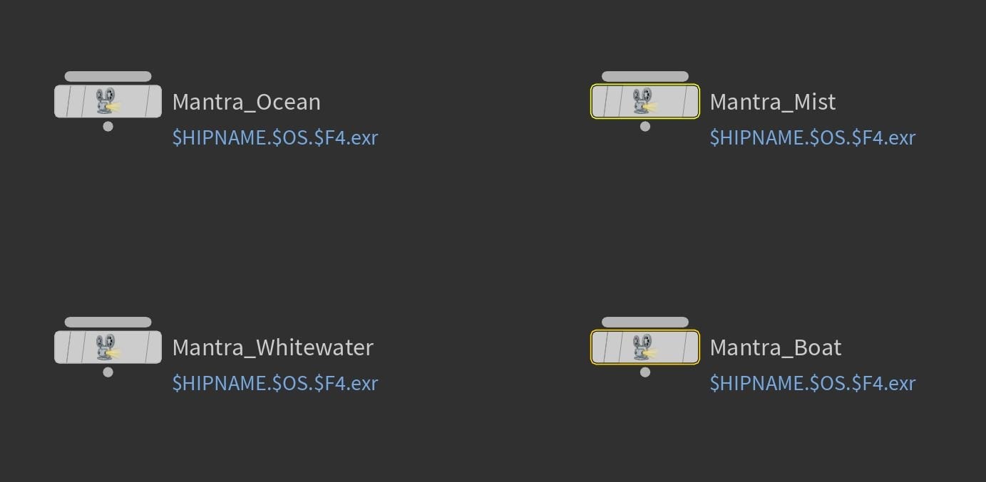
Our final out layer with all our Mantra nodes.
And we’re finished in Houdini, the last step is to make sure your Mantra nodes are set to render the whole frame range and then render out each Mantra node. They will take a variety of times to render out, the longest by far will be the Mantra Ocean as this is where the majority of our detail lies – it’s also very big.
Compositing
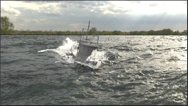
Giesen uses Nuke to composite his rendered layers however in truth you can use any video editing software, as this blog is predominantly about Houdini I will not be going into detail about how Giesen does all the things he does in Nuke in this post, just what they are. The layer order for your composition should go as follows: Ocean > Boat > Whitewater > Mist so that the Mist is on top and the Ocean is at the bottom. One important pass to add is a “depth pass” this will create a mask allowing you to blur the background and reduce the saturation accounting for distance. Another useful thing Giesen has done is exported the motion of the camera from Houdini, imported this into Nuke and applied it to the background layer he has created so the sky moves realistically with the rest of the shot. Lastly he adds a final layer of colour correction to get a nice filmic look for our shot.
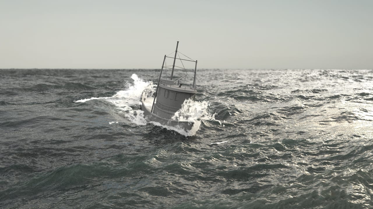
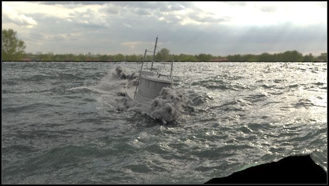
A single frame from my final render composited in Adobe Photoshop.
Conclusion
Well that’s it. We now have a completed realistic ocean shot. This has been a very long process (approximately 19,000 words if I’ve done the maths correctly) but I’m glad I took the time to write out the various steps to creating such a composition; now when I am creating my own similar shot instead of having to watch the tutorial series a third time I will hopefully be able to use my own posts as a guide and only refer to the videos occasionally. There are, of course, always further tweaks we could make to our shot and it will never be 100% perfect, but for our first one this is not bad by any means. My next step from here is to source some reference footage and a new boat object for my own stormy ocean shot, then begin the process again. For this however I will document my workflow in video form, potentially with my own narration over the top.
REFERENCES
- Pluralsight (2017) Houdini: Intermediate Ocean FX. Available from: https://app.pluralsight.com/library/courses/houdini-intermediate-ocean-fx/ [accessed 29 October 2018].