
Introduction
The first shot we are going to create to learn how to create a realistic pyro simulation is a campfire scene. Rickles provides all the scene files and the necessary geometry to begin with along with the course but the actual fire we will create ourselves.
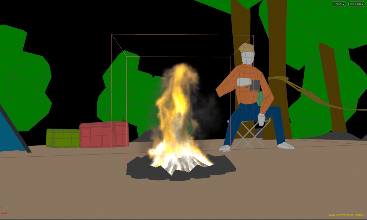
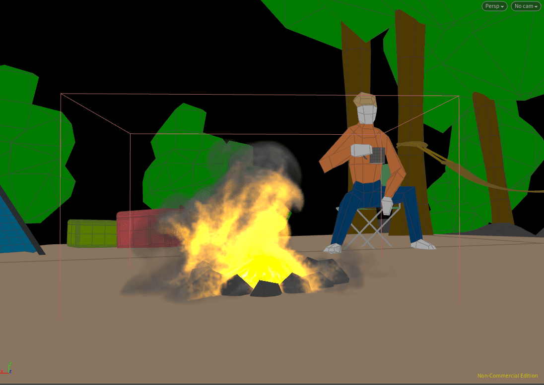
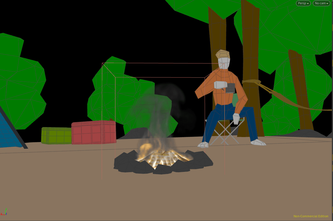
The opening campfire scene.
Starting with Fuel
First thing’s first, to create our pyro simulation we are going to need to create some fuel, to do this we are going to isolate the logs and turn them into fuel like we did with the sphere in the previous post. Firstly drop down a Geometry node to create a new network and rename it campfire_source. Get rid of the file node created automatically in the network and drop down an Object Merge node pointed at the object you want to use for your fuel – in this case the CAMPFIRE_GEO Null. Make sure the Transform is set to Into This Object so any transforms already applied will be brought in too.
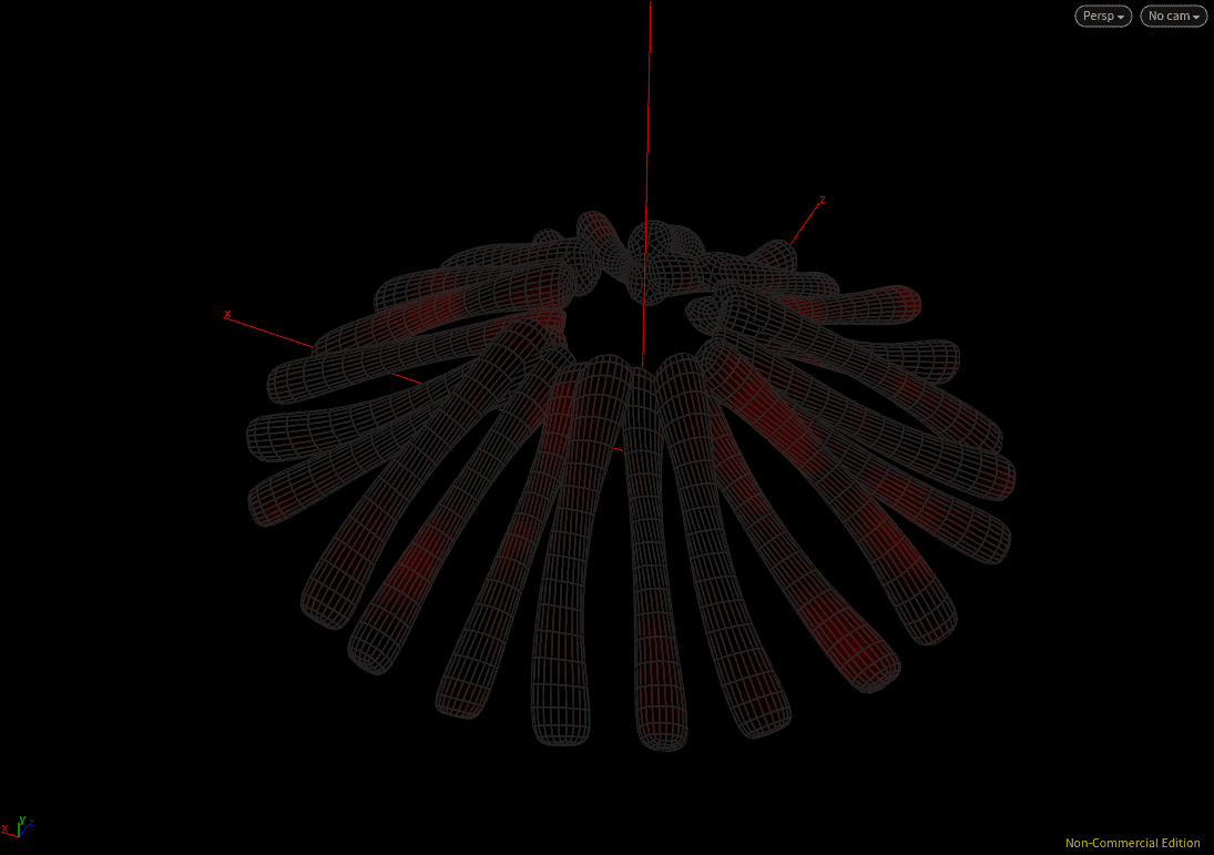
Currently we are importing in the entire scene, we just want the logs so connect a Delete node to the bottom of the Object Merge and set it to the campfire_wood group with Delete Non-Selected enabled. This will isolate just the logs in the campfire pit (if you’re creating your own scene you will need to set up these groups yourself). At the moment the logs are pretty low resolution due to the art style of the scene, we need a lot of voxels in our fuel creation to create high resolution fire so add a Subdivide to the bottom of the chain with a Depth of 2.
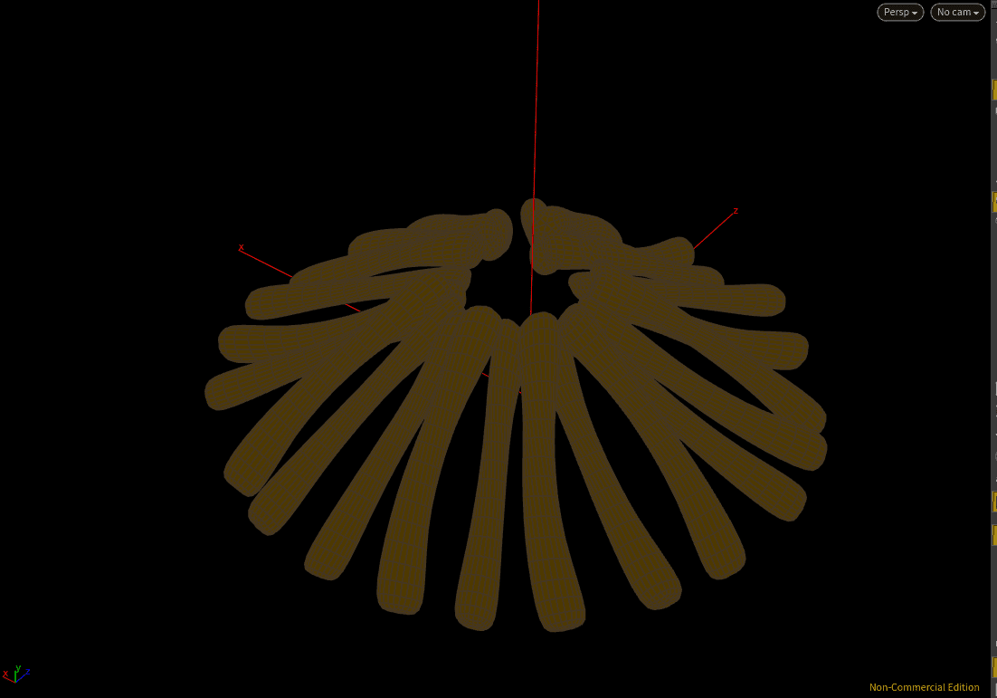
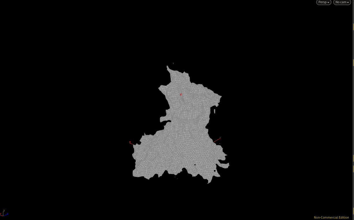
The isolated subdivided logs.
As I mentioned in the previous post, if we just turn the logs into big blocks of fuel then our fire will look very dull and not move much so we need to break up the volume somehow, we could just use the noise tab in the Fluid Source but instead Rickles uses a Point VOP in order to generate a “colour based noise” the effect of which should become clear as we go. Drop down a Point VOP and connect it to the chain via the input on the far left, then jump into the VOP Network. To create our noise drop down a Turbulent Noise node and connect the Point attribute (P) of our Geometry VOP Global to the pos attribute of the Turbulent Noise. We want to be able to control this noise from a level up so promote the Frequency, Offset and Amplitude parameters and you will now see them as sliders on the Point VOP node itself. We need a vector in order to generate the colour for our noise and as our noise is 1D we will use a Float To Vector node, connect the top input to the output of the Turbulent Noise and the FtV output to the colour (Cd) input of the VOP Output and you should see a change in your viewport.
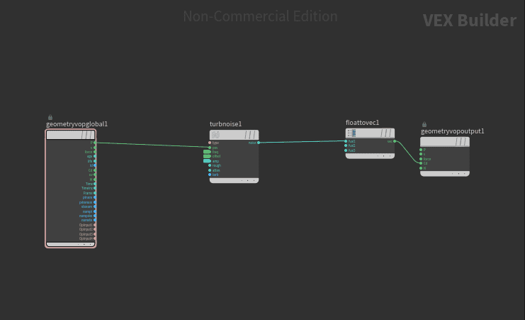
The interior of our Point VOP set up with the 3 promoted parameters.
This however is not the pattern we are looking for in our noise so head up a level and we will edit our promoted parameters. Firstly link your Frequency and Offset y and z values to the x value as we want them to always be the same then up your Frequency to 10 and you will start to see a bit more break up. However there is a bit too soft a falloff in the colour so, back in the Point VOP, add a Power node after the Turbulent Noise with the Exponent parameter promoted. If you increase this value to around 3 you will see that most of the colour has been deleted leaving only small areas left to burn which we can animate to move by giving the Offset a value of $T*10 which will change the value based on 10 times the time. Now if you play your timeline you will see the coloured areas moving around the logs at random. We only want to be using the coloured areas for our fuel, to isolate them add a Delete node to the bottom of the chain set to Delete By Expression with the expression $CR<.1 (all areas with a colour value less than 0.1 i.e. black areas).
Our subsequent log noise coloured red.
Now we need to turn this isolated colour into our source.To do this we will next need a Fluid Source connected to the bottom of the chain with the Container Settings set to Source Fuel. Now if you display the info panel you will see a Fuel and a Temperature attribute being created. Our fluid source is still far too low a resolution to be an effective source though so reduce the division size so that for both attributes there are around half a million voxels (Rickles uses 0.01). Next we need to refine the actual geometry of our source as there are currently just two blobs of smoke, to visualise these changes up the scale of both attributes to 100. Next, in the SDF From Geometry Tab, reduce the feather significantly to around 0.003 and increase the edge location by a few thousandths and our source geometry should already look bit better.
Finally, to get some interesting flames at the beginning of our simulation we will add some initial velocity to our fuel using the Curl Noise function in the Velocity Volumes tab. Enable the noise and reduce the Swirl Size by to about a quarter and that should be a good amount for the size of our campfire. Remember to reduce the scale of the Fuel and Temperature back down to 1 in the Scalar Volumes tab otherwise there will be far too much of both when we bring it into our DOP Network. Also, in preparation for the sim, connect a Bound node to the bottom of the Fluid Source with an Upper Padding value of 0.5, while not part of the main chain this will still help set up the bounding box in the pyro_sim network. Lastly add a Null to the bottom of the Fluid Source renamed to OUT_Source – this isn’t essential however I like to do it for neatness’ sake.
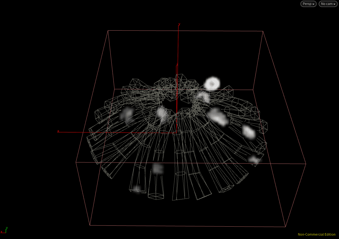
Our fuel source visualised against the templated geometry.
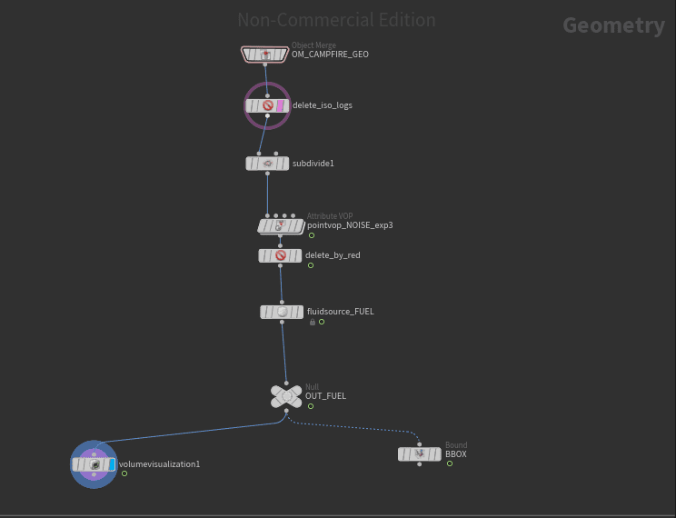
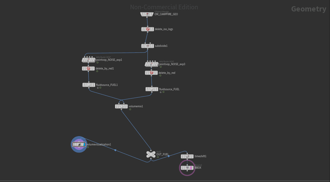
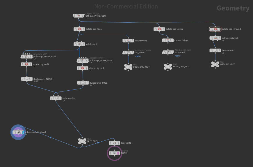
The campfire_source network currently.
Setting up the Fire
Rather than using the DOP Network Created by the shelf, Rickles shows us how to make one from scratch. Firstly, on the network level, drop down a brand new AutoDOPNetwork and rename it campfire_sim (or whatever you want to call it), inside there should already be an Output node set up. The first node we need is a Smoke Object so we can define the resolution and domain of our fire, then drop down a Pyro Solver, connect the Smoke Object to the far left input and the solver output to the Output node itself. We need to set our fire domain to cover the area defined by our campfire_souce, we can do this by linking the Size of our Smoke Object to that of bounding box in the source network. To do this we will use the expression:
bbox(“../../campfire_source/Bounding_Box”, D_XSIZE)
Here is the expression broken down:
bbox – Tells Houdini we want to create a bounding box we then have to present it with a string and a float.
“../../campfire_source/Bounding_Box” – This is our string or path, it tells Houdini where we want to source our bbox from. “../” means one directory up so we need two to go up once from the node, then again to the network view and “Bounding_Box” is what I renamed by Bound node to.
D_XSIZE – This is our float this tells Houdini what value you want to source for the bbox, for the x value of the Size use D_XSIZE and then change the letter for the corresponding y and z values.
We need to use a slightly different expression to also set the centre of our Smoke Object with is as follows:
centroid(“../../campfire_source/Bounding_Box”, 0)
For x use a value of 0, for y use 1 and for z use 2. This will point the centroid at the corresponding values and set the centre of the flames to that of the source.
Our simulation box with the linked Position and Centre parameters.
Next we need our actual fuel so drop down a Source Volume node connected to the 5th input of the solver. We are bringing in fuel so set the Initialise setting to Source Fuel then point the Volume Path to the OUT_Source Null we created in the campfire_source network. To visualise what our flames will look like toggle off the Density visualisation in the Smoke Object and enable Multi Field – we will then set up the Multi Field tab in the same way as the visualisation node in the last post. Currently nothing is still showing up because of our very low resolution, reduce the Div Size to something like 0.01 and enable Solve On Creation Frame or frame 1 will not be simulated.
Additional Fuel
At the moment we are creating no actual fire just sparks and a bit of smoke so we need some more fuel. To do this duplicate the Point VOP, Delete and Fluid Source nodes in the campfire_source and reduce the Exponent of the new Point VOP to 1. To combine these two fuels drop down a Volume Mix node and plug the original Fluid Source into the 1st input and the new one into the 2nd. Because we only want to be mixing the Fuel attribute as otherwise there will be far too much Temperature and everything will just ignite immediately so set the Source and Mix group to fuel using the drop down menu. Next change the Mix Method to Add so we are adding our new fuel on top of the old one, but we don’t want to add all of it or there’ll be too much so half the Source Pre-Mult to reduce this. Now move the Null over so it’s connected to the output of the Volume Mix and see how your simulation has been updated.
The campfire_source network with the added fuel branch.
Now we are generating a decent amount of fire.
Adding Collisions
Right now our smoke is just sort of spewing everywhere and moving through our wood and rocks, to fix this we will add some collision geometry to our source. As we’ve already isolated our logs with that first delete we will work from there, create a second chain by dropping down a Connectivity node and connecting it to the output of the first delete. In this node set the Connectivity Type to Primitive and it will group our connected primitives together. The reason we are doing this is because next we will use an Attribute Create node which can read this Class attribute. To do this, connect the Attribute create to the bottom of the new chain, set the Name to “name”, the Class to Primitive, the Type to String, and then in the string field type:
log_’$CLASS’
Now all our logs have been isolated from one another, we will turn this into an actual collider in the campfire_sim network so create another Null at the end of this chain named OUT_Collision.
To do this head over to the sim network and drop down an RBD Fractured Object node, this RBD can split up geometry by its name so is perfect for our purposes as we just assigned our geometry log names. In the SOP Path target the OUT_Collision Null and, using a Merge node below the Pyro Solver, merge in the RBD making sure it is the top Input Operator. As we only want this to exist as a collider disable Create Active Objects and our collision geometry is complete. Now we need to do the same process for our rocks.
You can duplicate the workflow we have just created, all you need to do this time is also duplicate the Delete node but this time point it towards the rocks rather than the logs. Also update the String in the Attribute Create so it says “rock_’$CLASS'” instead of log. Then just duplicate the RBD in the sim network and update it to the rocks’ OUT Null.
Lastly we need a ground plane. Back in the source network duplicate the Delete again and update the path so it points at the ground. We want to turn this into a volume and for that we’ll need depth so connect an Extrude Volume node to the bottom of the new Delete with a Depth of -1. By connecting a Fluid Source to the bottom of the extrude and setting the Container Settings to Initialise: Collision. Again we need a Null and name it appropriately before hopping over to the campfire_sim again and creating another Source Volume to bring in the ground plane. Initialise: Collision again and then point the SOP Path to the ground plane Null, Source Volumes plug in to the 5th input on the Solver but we already have one plugged in there so create another Merge and connect it up to the chain with both Source Volumes connected to the input.
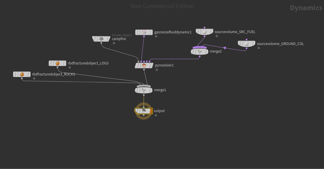
Our DOP Network with the added collisions.
The last step before we refine the look of our fire is to create our dynamic bounding box. To do this drop a Gas Resize Fluid Dynamic node in the campfire_sim network and connect it to the solver via the 2nd input. Then, in the Max Bounds tab just disable the Clamp To Maximum option. We don’t want the box to be too big or we will be wasting calculation time so reduce the Lower Padding in the y axis to 0.05 as our ground plane will be blocking this anyway and also reduce the Padding to 0.1 as this is only a campfire and therefore shouldn’t be too crazy.
Our fire is looking pretty weak at the moment.
Refining the Fire
Final Source Modifications
There are a number of problems we need to fix before we cans stylise the fire, firstly the bounding box in the first few frames is a bit all over the place until the fire kicks in – this can be fixed in our source. If you switch round the inputs of the Volume Mix this can be accomplished however now the fuel with the animated noise is being added onto the big fuel so we need to change some parameters in the Mix compensate. All we have to do is swap the values of the Dest and Source Pre-Mult and the same effect can be achieved. Now we have another issue though, the temperature and velocity are now being taken from the broader fuel source rather than the one with the noise meaning there will be far too much of both so we need to isolate some fields. Connect a Delete node to the output of the first Fluid Source we created and set the Group to fuel from the dropdown menu, then duplicate and invert this by changing the Operation to Delete Non Selected and placing the duplicated node between the Volume Mix and the OUT_Source node. Lastly drop a Merge node before the Null and connect both Deletes to the input, to check this has worked look at the info panel and compare it to your earlier values.
Our final campfire_source network.
Our source is slowing down our simulation a bit at the moment, this is because of the broad fuel created by our second Fluid Source. As we are only use this to add a base layer of fuel to our source we can afford to decrease the resolution by increasing the Div Size to 0.02, now play your timeline and it should run smoothly. Our fuel is also moving a bit fast for such a scene so reduce the Offset multiplier of our Point VOP from 10 to 1 and we will see a much more gradual transition in our noise.
Tweaking the campfire_sim
As we are going to be doing a lot of testing of our simulation add a multiplier of 2.5 to the division size to significantly decrease the resolution but increase simulation speed.
To actually stylise our fire we are going to be working in the Combustion tab of the Pyro Solver, set the Burn Rate to 1 and the Fuel Efficiency to 0 so that no fuel is being wasted in the burn. If you play the timeline here you should see we already have a bit more fire being generated and then a decent sized explosion of flame – this is not the look we are going for. This fireball has been created because we are releasing too much gas in our fire so reduce the Gas Released to something like 4 and now when we hit that temperature threshold that ignites a lot of the fuel there is still a sharp increase in flames, but not to nearly the same extent. To get rid of this explosion effect completely set the Temperature Output to something like 4, that way in the first couple of frames the fuel will all be ingnited and then we will have a much more controlled fire. Lastly we will make our fire a bit taller by increasing the Flame Height from 3 to 15 which should fit our purposes nicely.
Now your flames should look something like this.
The fire is sticking together a bit too much at the moment and we aren’t getting many of this interesting flame licks that we are looking for so we need to make a few more tweaks. Firstly in the Simulation tab reduce the Temperature Diffusion to 0.05, this will stop Temperature from collecting in certain areas and brake up our flames a bit. This has made our fire much to tall so to counteract this we will increase our cooling rate to 0.94 so temperature is rapidly lost and our flames turn to smoke before they can get too high.
Our final level of stylising will be added in the Shape tab, Rickles warns against using the parameters in this tab to drive the look of your fire as they are very large and resource intensive. Instead it is recommended to get a good base, as we have done, in the Simulation and Combustion tabs before moving over to the Shape tab to add some finer detail – we have used this workflow and are now ready to play with the shape tab.
Firstly we will enable Disturbance adding a lot of high frequency noise and breaking up the flames. By default this effect will be far too strong so reduce the Block Size to 0.01 to make the disturbance more subtle. We’re also going to enable the Sharpening option to promote more wispy, broken flames in our simulation, rather than large clumps.
As Rickles puts it, if new play our simulation, currently our campfire looks a bit too much of an inferno at the moment for a calm campfire scene. To rectify this we will lower the Timescale to 0.7 which will really scale down our fire. The simulation step of our scene is now finished and we are ready to prep the shot for render, if you are happy with the look of your fire you can now remove that Division Size multiplier to achieve the maximum resolution.
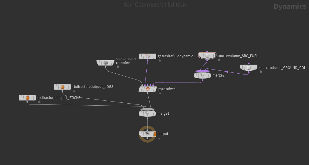
The final campfire_sim network.

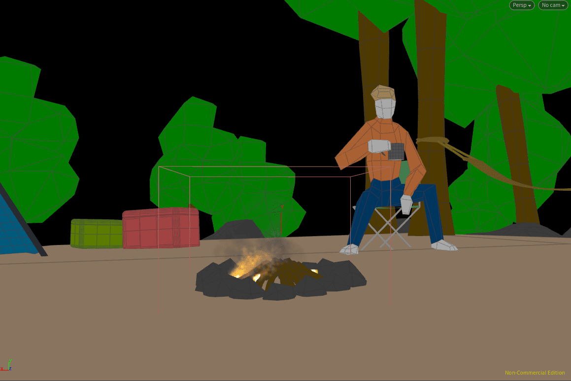
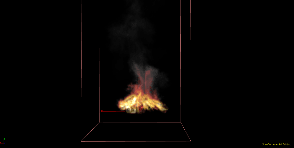
Our fire at the end of the simulation stage.
Fire Exporting
As we are creating our pyro networks from scratch we need to create another new Geometry network to take the data from the simulation and prep it for render so drop one in the network context and rename it to campfire_import.
Within this network we need to drop a DOP Import Fields node that will import all the data from the Output node in our campfire_sim. First we need to point the Import at our DOP Network so set that field to your campfire_sim network, then set the DOP Node field to the Smoke Object within that network. Finally, set the Preset to Pyro so that the correct fields will be imported, if you display the info panel for the node now, you will see all the attributes that have been imported. In order to actually see your fire connect a Volume Visualisation node to the bottom of the DOP Import and set it up like we did in the previous post.
To actually cache the simulation just connect a ROP Output to the bottom of the chain, update the path as we have done before and then Save To Disk. To import this data back in drop down a File node and browse for the output cache. For neatness’ sake I again recommend adding a Null to the bottom of this chain named appropriately so we can target that when we come to rendering.
Our final visualised fire.
Embers
Watching our cached fire back it looks like it could do with one extra layer of detail, floating embers. Fortunately we will not have to re-cache our fire to do this, we can build them separately, starting with a new Geometry network on our object layer that I will rename campfire_embers.
Firstly, using an Object Merge, bring in the cached out fire by targeting the Null in the campfire_import. To create embers we will need geometry and velocity, fortunately we can get both of these from the attributes of the fire we have already exported. Isolate the Density of the fire by using a Delete node with the Group set to Density and Delete Non-Selected enabled. Now we have a volume we need to turn it into a geometry, connect a Convert VDB to the Delete node via the 1st input and set the Convert To to VDB and the VDB Class to Fog to SDF. Next connect another Convert VDB to the bottom of the chain, this time with the Convert To set to Polygons. At the moment nothing is visible however if you drop a Volume Mix directly below the Delete with the Source Pre-Mult set to 10 you will see the density of the fire represented in geometry.
We have now created a mesh from our flames.
We also need to isolate the velocity so create a new chain coming off the Object Merge with a new Delete Non-Selected Delete node pointed this time at the velocity, change the group so it say @name=velocity.* though so it brings in the x, y and z velocity values.
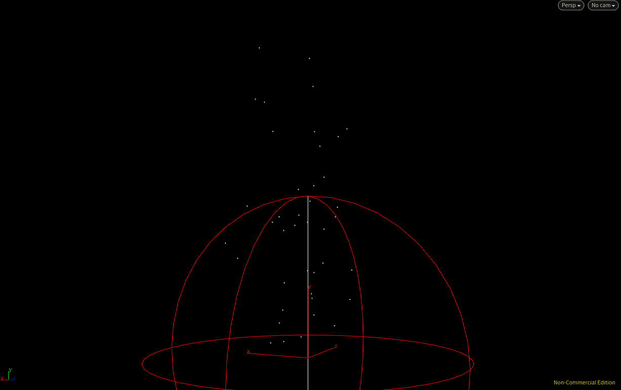
To advect our embers we are going to use a POP Network, plug the geometry chain into the 1st input and the isolate velocity into the 2nd, then jump into the POP Network. This should look pretty familiar from our simulation networks and it is essentially the same set up. If you play the timeline then you will see particles are being generated off our fire geometry which is exactly what we want but there are far too many being created at the moment so in the Birth tab of the POP Object reduce the Const. Birth Rate to 20 and the Life Expectancy to 2 with a Life Variance of 1 so the embers only exist for a few seconds before disappearing.
At the moment our embers are just sort of sitting still so we will add some initial velocity using the Attributes tab of the POP Source. We want to supplement the velocity we already have so set the Initial Velocity to Add To Inherited Velocity. Set the Velocity to 0, 0.25, 0 as we just want our embers to rise, but give it an x y and z Variance of 0.1 each so all the particles do not have exactly the same motion. If you disable the guide so only the embers are visible and play the timeline our particles are starting to look good.
We still need to bring in the velocity from our fire so drop down a POP Advect between the source_first_import and the wire_pops_into_here. As we plugged our isolated velocity into the 2nd input change the Velocity Source to Second Context Geometry. Increase the scale to 2 and play your timeline and you’ll see our embers are starting to pick up speed in certain areas as they are advected by the velocity field.
Lastly, to add another layer of realism we are going to make our embers spin around our fire using a POP Axis Force. Drop this node below the POP Advect and increase the Orbit Speed to 3 in the Speed tab. If we play our timeline now our particles are moving in a subtle but circular motion.
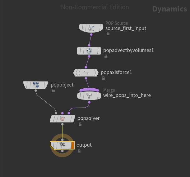
The embers DOP Network.
The viewport with the added circular motion.
Jump up a level back to the embers network, at the moment we are just creating points and no actual geometry will be rendered. Firstly we are going to colour particles by age, drop down a Colour node under the POP Network with the Colour Type set to Ramp From Attribute and the Attribute field set to “age”. To make this look a bit more like fire change the colour values so at the beginning of the ramp the particles are yellow and the end they are red meaning that as particles age they will appear to lose their temperature.
Next we need to make our particles fade rather than just disappear, to do this we will manipulate the alpha of our particles. Drop down a Point node at the end of the chain, change Keep Alpha to Add Alpha. In the actual Alpha field use the expression “1-$LIFE” which means as the life (how long the particle has existed) increases the Alpha will decrease until the particle disappears.
Finally, to get our embers to render properly we need to give them some geometry. Drop a Copy node at the bottom of the chain but connected to the 2nd input so we are using the chain as the template, then connect a Sphere node to the 1st input which will map a sphere to each particle. The spheres are massive initially so reduce the Uniform Scale to 0.003 so they are small enough to look like embers also, in the Copy node toggle on Use Template Point Attributes and the colour ramp will be added to the spheres.
Drop a Null at the end of the chain and name it appropriately then head back to the network layer and we can preview our shot. We are now ready to prep the scene for rendering and export it using mantra.
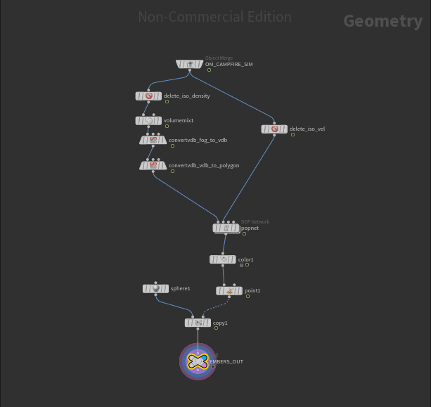
Our final campfire_embers network.
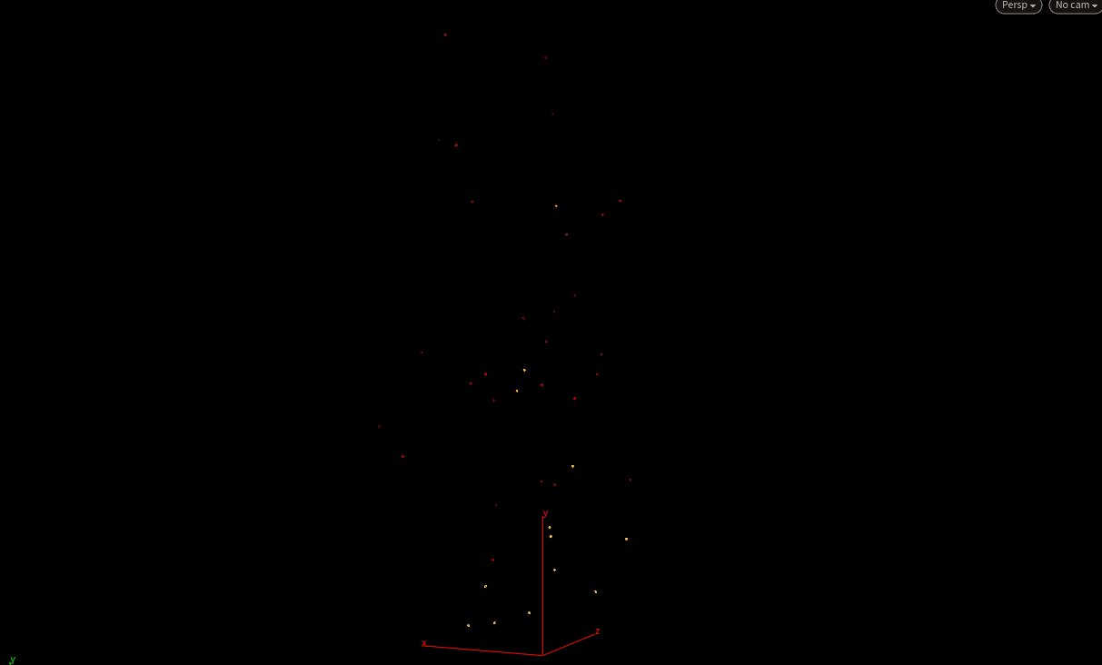
Our embers visualised in the viewport.
REFERENCES
- Pluralsight (2016) Introduction to Houdini Pyro FX. Available from: https://app.pluralsight.com/library/courses/introduction-houdini-pyro-2504 [accessed 16th November 2018].