
Introduction
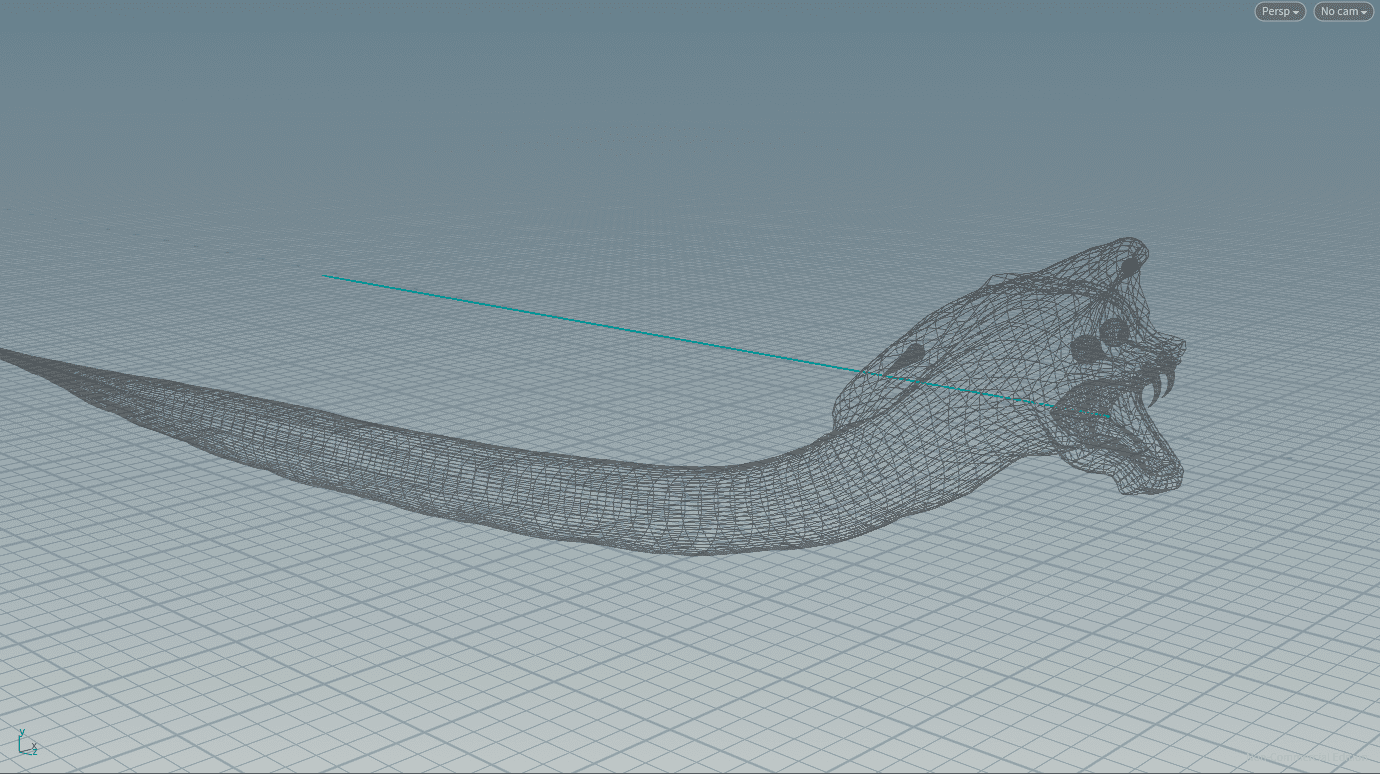
Now we have completed our campfire scene we will move onto a more complex scene that we might use in a film, a fire breath effect. Rickles gives us the initial geometry to create a shot where a snake breathes fire onto an unsuspecting figure which I will discuss the steps to create in this post.
Creating the source
Point Isolation
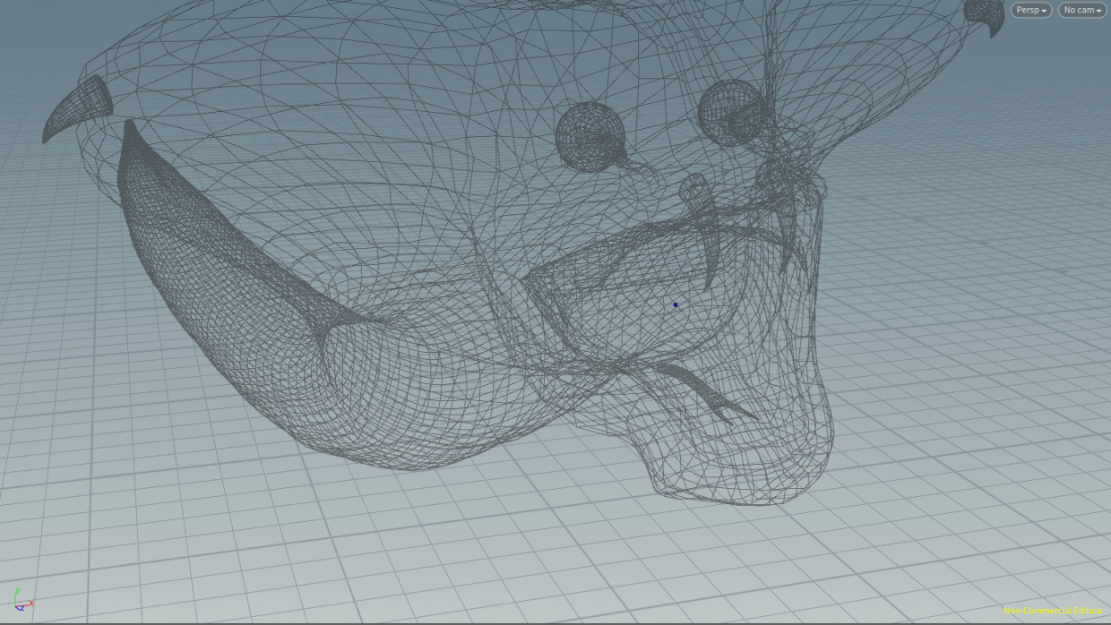
As our snake is moving and will be expelling the fire from its mouth we can’t just set the snake as the source for our fire, we first will need to isolate the mouth from the rest of the snake’s body and then create an emitter mapped to that isolated mouth so fuel will be expelled from the snake’s mouth just like a flamethrower in real life.
Firstly we need a new geometry network (renamed to snakefire_source) with an Object Merge at the top bringing in our Snake Geometry “Into This Object”. At the moment our snake is being brought in as a “Polygon Soup” and we need it to be just polygons so we can isolate the mouth so connect a Convert node to the bottom of the chain which will, by default, convert to polygons. Similar to our campfire we are going to use colour to isolate our mouth so drop down a Colour node at the bottom of the chain set to change the snake colour to black. Then connect a Paint node below that with the colour set to red (or any block colour) and we will isolate our mouth in the viewport by spray painting the entire interior of the mouth. Then, to group this painted area connect a Group node set to Points and Group By Expression with that expression set to $CR>0.2 which will group any points that aren’t black.
We only want the mouth group for our emitter so isolate it with a Delete node set to Entity: Points. To create our Emitter we need to locate a centre point in the mouth, drop a Null at the end of the chain named “Mouth” and then a Point node below that with this expression in the x, y and z values:
centroid(“../Mouth”, 0)
centroid(“../Mouth”, 1)
centroid(“../Mouth”, 2)
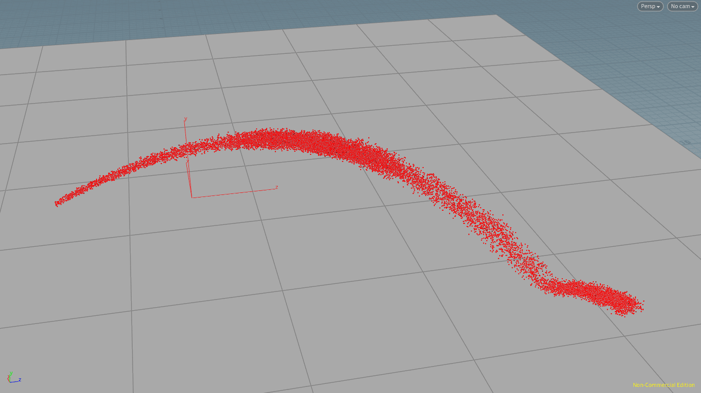
The isolated throat emission point.
Creating a Velocity Vector
This expression will generate a single point at the very centre of our mouth which we can then use to emit fuel. The last step before we set up this fuel emitter is to refine the normal of this emission point. When we emit our fuel we need it to emit with velocity, the direction of which will be defined by the point normal, now the point will have a normal already based off of all the normal value of the other points in our isolated mouth. Because these normals will all be pointing in different directions we need to set our emission point normal ourselves.
The snake geometry already has the tongue group isolated which is conveniently pointing straight of the mouth in the direction we want for our normal so create another Delete node isolating the tongue starting a new chain after the OM. Plug a Box node into the bottom of this Delete and it will surround the tongue geometry with a box, to work out the normals we need to isolate the two primitive at the front and back of the tongue box – to do this we will need two more Delete nodes, creating two separate subchains, isolating a face each using the Delete by Pattern Operation. To figure out the vector between the two faces use a Point Wrangle with the front face plugged into input 1 and the back face in input 2, then enter this VEXpression in the field to calculate the vector:
vector P2 = point(1, “P”, @ptnum);
v@v=P2-@P;
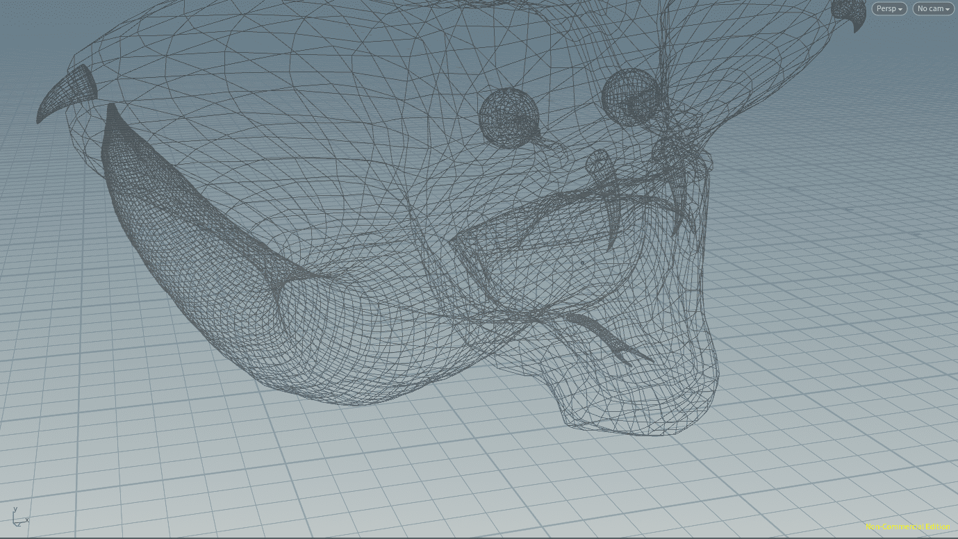
We now have a velocity vector ready to apply to our emission point, to do this drop down an Attribute Transfer with the first chain plugged into the 1st input, and the 2nd into the 2nd. Disable Primitives and increase the Distance Threshold to 100 so our point is in range and now if you display velocity in the viewport you will see our point has our velocity vector applied to it.
The point with the velocity vector mapped to it.
Creating an Emitter
We’ll use another POP Network to create our emitter so drop one at the bottom of the source network connected to the first input. We don’t want the emission to start until the snake opens it’s mouth so in the POP Network>Simulation tab set the initial frame to that point (60 for me). If we dive into the POP Network we need to make a couple of initial tweaks, firstly change the Emission Type in the Source_First_Input to Points, and we need to make sure we are simulating gravity by dropping a Gravity node above the Output. We also need a Ground Plane node connected to a Merge node below the Gravity so our fuel doesn’t just fall forever.
What should be immediately obvious if we play our timeline is that there is not nearly enough initial velocity being given to our points as they are just sort of spilling out of the snake’s mouth at the moment. Jump a level and drop a Point Wrangle above the POP Network with this VEXpression:
v@v*=30;
Which just means the velocity value at the vector should be multiplied by 30. Now when we play our timeline has much more velocity and is looking a little better but very uniform. We need to add some variance back in our POP Network in the Source_First_Input node change the Initial Velocity to Add to Inherited Velocity and give it an x, y, z variance of 0.5 each. Now we have much more of a cone shape when we play our timeline.
At the moment our particles are living forever and are being expelled at a constant rate which will give us some very boring fire, in the Birth tab of the Source_First_Input this can be fixed. First set the Const. Activation to $FF<=106 as the snake has closed its mouth at this point, also reduce the Life Expectancy to something like 0.9 with a Variance of 0.4 so the particles disappear before they even reach the ground. By default the Const. Birth Rate is set to 5000 however using a Sin function we can get a fluctuating level of emission, the expression we need to enter is:
fit(sin($FF*30), 0, 1, 1000, 5000)*10
Lets break down this expression.
sin($FF*30) – $FF represents the current frame and *30 will times that frame number by 30. By placing this calculation as a sin function a value between 0 and 1 will be generated, if we look at a sin graph we can see how.
As the value between the brackets gets closer to 90/270/450… a value nearer 1 will be output and then as we move closer to 0/180/360… a value closer to 0 will be output.
0, 1, 1000, 5000 – This is a way of mapping points to values for the Const. Birth Rate, what these specific values are saying is that if the value of the sin function is 0 then the Const. Birth Rate should be 1000 and as this value increases to 1 increase the Birth Rate to 5000.
*10 – Our particle emission looks a little bit like stairs, using this multiplier we will over sample the birth rate and break this up a little.
Now as our timelines moves along the Birth Rate will fluctuate between 1000 and 5000 breaking up the uniformity of the emission.
Our fuel needs a little bump to the y velocity just to help the effect of it being fired out of the snake’s mouth so in the Source_First_Input>Attributes tab increase the y-velocity to 0.5. To break up the “stepiness” I mentioned before we are going to simulate some wind using a POP Wind below the Source_First_Input. We want this to be subtle so reduce the Air Resistance to 0.2, give it an Amplitude of 1 but a Swirl Size of only 0.1. If you hop up a layer and change the Sub Steps of the POP Network to 4 then play the timeline now a lot of that “stepiness” will be gone.
Looking at the viewport it looks like the emission could do with a bit more z velocity just to force it out that little extra bit further. In the Point Wrangle add a second line of VEX:
v@v.z*=2
This will fire the fuel a bit further from the snake.
The points emitted by our Point VOP.
Creating Fuel from the EMITTER
We next need to isolate the points from the simulation so drop another Delete after the POP Network isolating the Points of the stream_source_first_input. As we did with the campfire we will use colour to drive the source so connect a Point node below the Delete set to Add Colour, we want the colour value to increase based on how long the particle has existed so in the Red and Green channel set the value to $LIFE – now new particles will be black and old ones will be bright yellow.
To create a pyro simulation remember we need Fuel so connect an Attribute Create to the bottom of the chain with the Name set to “fuel” and a Value of $Cr (referencing the red colour channel). We also need to create Temperature so duplicate the Attribute Create and set the Name to “temperature” and this time use a Value of $Cg (referencing the green colour channel). To turn these attributes into a source connect a Fluid Source node to the bottom of the chain with the Method set to Stamp Points – we now have a visualisation of our fuel. We are creating fuel so in the Container Settings set the node to Initialise a Source Fuel and we have a gradient from the beginning of the particle simulation to the end of it thanks to the conditions we set up in the Attribute Creates.
We want this gradient to be a bit faster however so the fire is pretty much at full capacity immediately after it leaves the snake’s mouth so we will update the expression in the Point node where we coloured in our points. Instead of $LIFE, instead use this condition:
if($LIFE>0.05, 1, fit($LIFE, 0, 0.05, 0, 1))
This expression means that if the particle is in the seconds 95% of its life it will have a colour value of 1, if however it is in the first 5% it will have a value between 0 and 1 based on how long the particle has been alive. Duplicate this for the Green value as well.
Next we are gonna modify the look of our fuel in the Stamp Points tab of the Source Fluid. We want fuel to be generated very close to our individual points so reduce the sample distance down to 0.03, however we want each point’s fuel to be quite dense so decrease the Threshold to 0.25. We want to be generating about 3 million voxels at the mid point of the emission so check your info panel and adjust the Division Size accordingly (0.03 in my case).
After this we will edit our noise so it has a bit more influence and breaks up our fuel emission a bit. The first step is to decrease the Element Size to around 0.2 and increase the Sharpness to around 0.6 so we get a nice harsh breakup. The next step is, in the Velocity Volumes tab, enable Curl Noise but with a reduced Swirl Size of only around 0.15 as we have a very thin jet of fuel. At this point, if you are happy with your fuel so far, we can afford to cache out our source up to now using a File Cache. Update the path and set the Frame Range so it only covers the area that fuel is actually generated in, toggle on Initialise Simulation OPs and then cache out the file using a File node after to bring the cache back in connected to a Null as we are done with this chain.
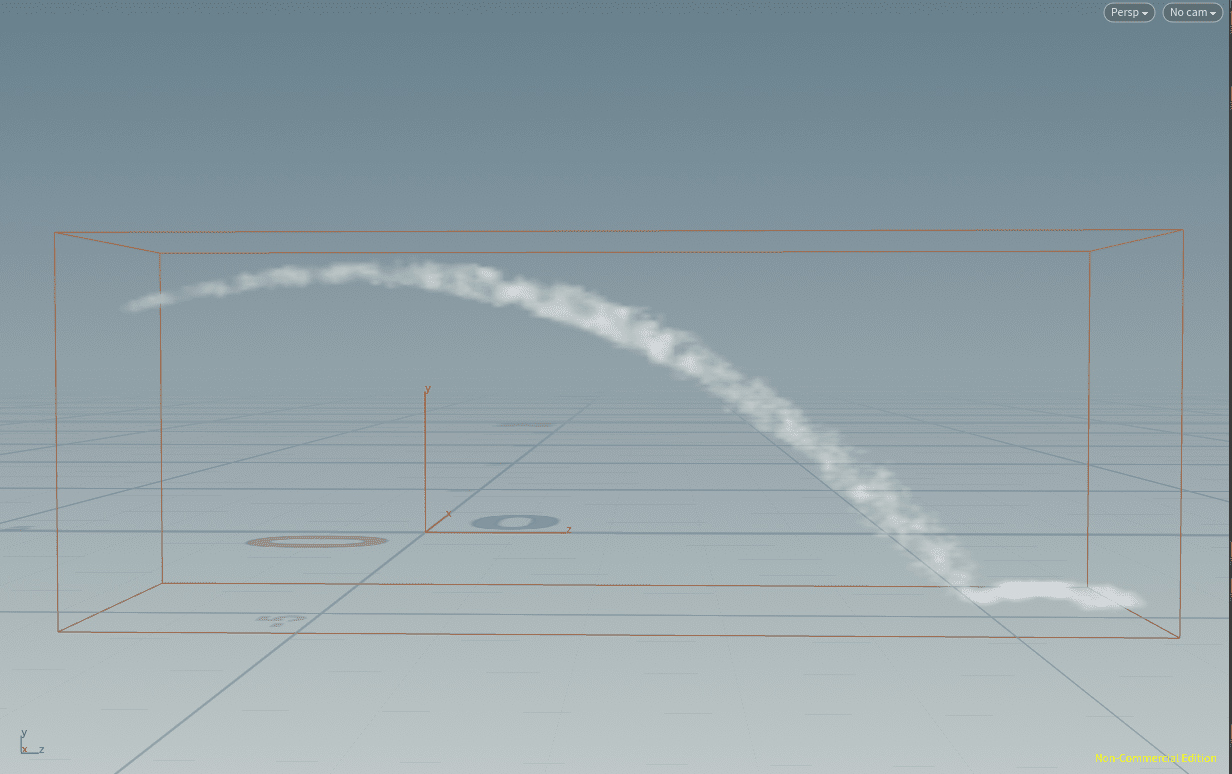
The final snakefire_source fuel.
Collisions
We need to isolate the head of the snake so no fuel is clipping through it so create another branch coming off the Convert node with a Delete node this time isolating the snake body group. We need to create our own group for the head, it doesn’t need to be too specific so just drag a box around the head/neck in the viewport and hit the Delete key which will create a Blast node after the Delete – enable Delete Non-Selected and we have our isolated head. At the moment there is a hole where we decapitated our snake so drop a Poly Cap node below the blast which will connect the geometry for us, next we need another Fluid Source to turn the isolated geometry into collisions. Make sure the Container Settings are set to Initialise Collision and reduce the Division Size down to something like 0.06 to increase the Voxel Count to around 150,000. To further refine our collision we need to reduce the Edge Location but in order to do that we first need to disable Output SDF then reduce the EL slightly to something like -0.03. Now we’ve finished our collision geometry so round of the chain with a Null.
The second collision we need to set up is the figure who will be set on fire. Create a new chain in the network with a brand new Object Merge this time importing the reference figure. Fortunately he’s already a geometry object so all we have to do is plug the OM into a duplicate of the Fluid Source we just created. Reset the Edge Location to 0 and increase the Division Size to 0.03 however so we have a more accurate model then just connect another Null to the bottom of the new chain.
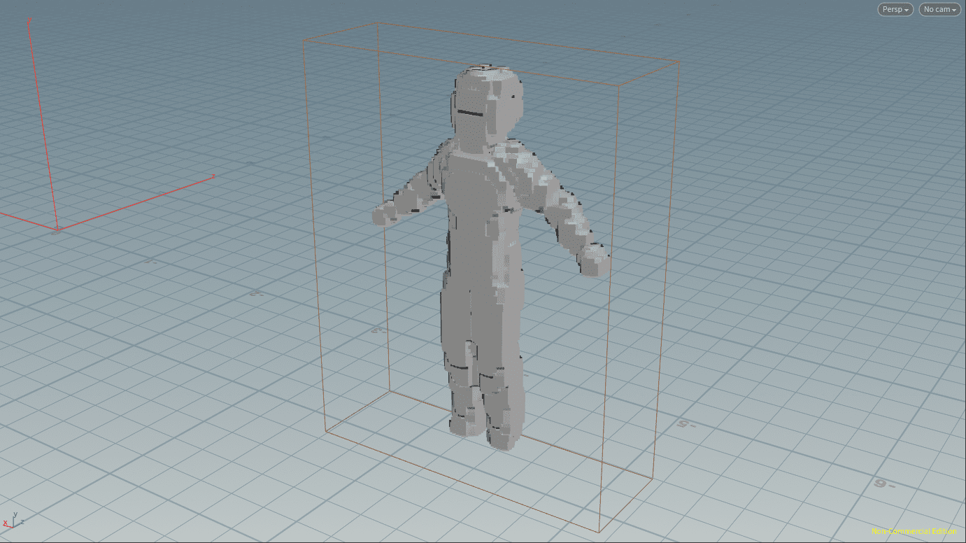
The collision geometry for our reference figure.
Bounding Box
Like in the campfire we need to set up a Bound node to prepare for the bounding box later so drop one down creating a new branch off the File node bringing in our cache and follow that with a Null renamed to BBOX so we can reference it later. To help the resize container later we are going to also add a tracking object so duplicate the Bound and Null but rename the Null to TRACKER.
We only need the box being simulated from frame 60 onwards drop down a Time Shift between the first Bound and Null and Delete the Frame channel so it has a value of 60 not referencing anything. You can duplicate this node and place it before the Null for the figure collision as well. Finally increase the Upper and Lower Padding of the first Bound node to 0.5 in all values just so on the first frame there is enough of a volume being simulated.
We now have our full source network ready to be simulated and turned into fire in the next stage.
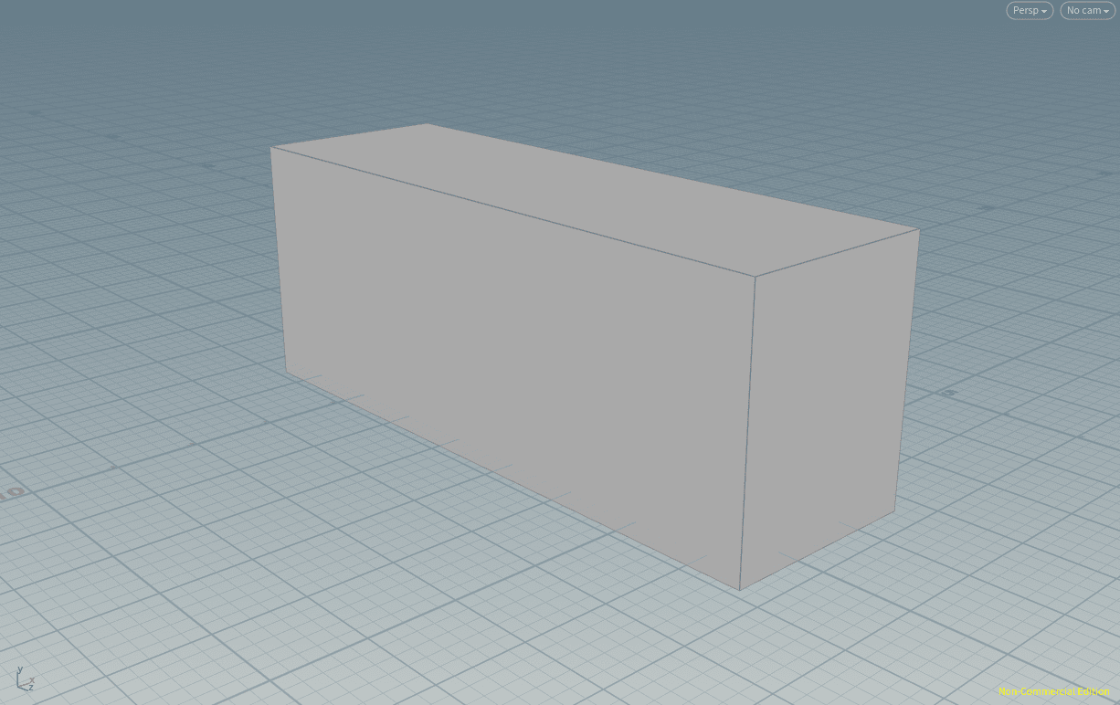
The source bounding box.
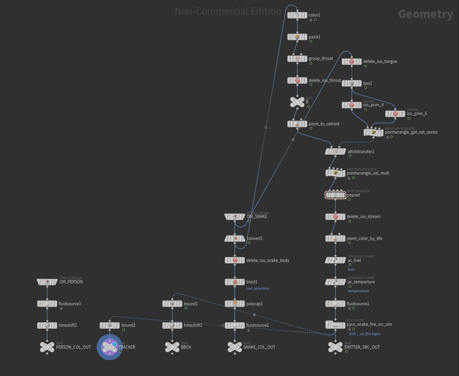
The final snakefire_source network view.
REFERENCES
- Pluralsight (2016) Introduction to Houdini Pyro FX. Available from: https://app.pluralsight.com/library/courses/introduction-houdini-pyro-2504 [accessed 19th November 2018].
- Isak, J. (2008) Maths Scene – Trigonometry Functions. Available from http://www.rasmus.is/uk/t/F/Su36k03.htm [accessed 19th November 2018].